YouZum

AI

AI, Committee, Noticias, Uncategorized

Black Forest Labs Releases FLUX 3: A Multimodal Flow Model for Image, Video, Audio and Robot Action Prediction

Black Forest Labs (BFL) has released FLUX 3, a multimodal foundation model that learns from images, videos and audio inside a single architecture. It is also the first FLUX model to ship video, audio and action prediction from one set of weights. The Black Forest Labs (BFL) research team argues that no single modality gives a complete description of the world. Images capture spatial structure at one instant. Video restores time and exposes physical dynamics. Audio reveals causal relationships between mechanical events and sound. Each is treated as a lossy projection of the same underlying reality. Training on all of them at once means the modalities constrain each other. The sound has to match the impact. The motion has to obey the mass. The research team calls FLUX 3 its first model built entirely on that principle. The method underneath: Self-Flow FLUX 3 builds on Self-Flow, BFL’s method for aligning multimodal generation and understanding in one architecture. Self-Flow combines the flow matching objective with a self-supervised feature reconstruction objective. The reference implementation on GitHub is Apache-2.0 and uses SiT-XL/2 with per-token timestep conditioning. It trains with a 25% per-token mask ratio and self-distillation from an EMA teacher at layer 20 to a student at layer 8. That released checkpoint is an ImageNet 256×256 research model, not FLUX 3. BFL states that it ‘significantly scaled up compute and data resources’ on the same approach to train FLUX 3 across video, images and audio simultaneously. Self-Flow itself was introduced in March 2026, so it is not new to this launch. What is new is the scale. What FLUX 3 Video does FLUX 3 Video generates clips up to 20 seconds long in a single generation, with native audio. The supported modes cover text-to-video, image-to-video, video-to-video from a reference clip, keyframe-to-video for controlled transitions, and generative video-audio continuation from input video and audio. BFL also lists multilingual dialogue, agentic chaining of clips into multi-shot sequences, and strong typography generation with animated designs. The BFL team reports particular strength in human facial expressions and in associating sounds with physical events. Performance BFL team published preliminary human preference results. The setup was 10-second text-to-video clips at 720p with audio. FLUX 3 was preferred over Luma Ray 3.2 in 93% of comparisons and over Runway Gen-4.5 in 77%. Against Grok Imagine Video the figure is up to 69%, then Kling v3 Pro at 60%, Happy Horse v1 at 59% and Happy Horse 1.1 at 57%. Against Seedance 2.0 and Gemini Omni Flash the result is 52%, close to a coin flip. Interactive Explorer bfl@flux-3:~/real-world-models Early Access Commands >spec >bench >compute >action >mimic >rollout >selfflow Type a command below, or press ↑ / ↓ in the prompt to cycle history. Every figure is sourced from Black Forest Labs or mimic robotics. flux3 $ Enter a command enter Sources: bfl.ai/blog/flux-3 · bfl.ai/blog/flux-3-mimic · mimicrobotics.com · figures dated 23 Jul 2026 Built by Marktechpost

Black Forest Labs Releases FLUX 3: A Multimodal Flow Model for Image, Video, Audio and Robot Action Prediction Leer entrada »

AI, Committee, Noticias, Uncategorized

Meet the New Claude Opus 5: Frontier-Class Agentic Coding and Computer Use at Unchanged Opus Pricing

Today, Anthropic released Claude Opus 5. It replaces Claude Opus 4.8 as the Opus-tier flagship. Pricing is unchanged at $5 per million input tokens and $25 per million output tokens. The Anthropic team positions Opus 5 as approaching the intelligence of Claude Fable 5 at half the price. It is now the default model on Claude Max and the strongest model on Claude Pro. What actually changed at the API level Three changes are quite important before any benchmark does: Thinking is on by default. On Opus 4.8, requests ran without thinking unless you set thinking: {“type”: “adaptive”}. On Opus 5 the same request thinks, and the effort parameter controls depth. Because max_tokens caps thinking plus response text, existing values need review. There is a breaking change. Setting thinking: {“type”: “disabled”} with effort xhigh or max now returns a 400 error. The restriction is enforced per request. You either cap effort at high or drop the thinking field. Anthropic tells developers to delete their verification prompts. Instructions like “include a final verification step” now cause over-verification, because the model already verifies its own work. The Opus 5 prompting guide covers the tuning patterns. The model ID is claude-opus-5. Context is 1M tokens as both default and maximum, with no smaller variant. Maximum output is 128k tokens on the synchronous Messages API. The Message Batches API reaches 300k with the output-300k-2026-03-24 beta header. The minimum cacheable prompt drops to 512 tokens, down from 1,024. Coding and agentic results On FrontierBench v0.1, a 74-task successor to Terminal-Bench 2.1, Opus 5 scored 43.3% at max effort. Opus 4.8 scored 18.7%. Fable 5 reached 33.7% and GPT-5.6 Sol reached 37.5%. At xhigh effort Opus 5 reaches 44.4% mean reward, its best result. One detail from that run is worth noting. Opus 5 safety classifiers flagged and refused 5% of API calls, across 4% of trials. Fable 5 classifiers flagged 42% of calls across 26% of trials. Opus 5 scored 96.0% on SWE-bench Verified and 79.2% on SWE-bench Pro. Fable 5 still edges it on Pro at 80.0%. On SWE-bench Multimodal the jump is larger, from 38.4% to 59.4%. The agentic numbers are the clearest wins. Opus 5 reached 70.57% on OSWorld 2.0 against 55.7% for Opus 4.8. On Zapier AutomationBench it scored 26.0%, against 17.0% for Opus 4.8 and 17.4% for Fable 5. At medium effort it still scores 24% at $0.89 per task. On Artificial Analysis GDPval-AA v2, Opus 5 takes the top two leaderboard spots at ELO 1861 and 1827. The xhigh setting beats every other model while using 25% fewer output tokens than max. Reasoning, and the ARC-AGI-3 result Anthropic prompted Opus 5 on all six IMO 2026 problems without tools or an agent harness. A three-model judge panel scored all 24 generated solutions correct. Human experts independently graded one pre-specified solution per problem at 7/7. The final 42/42 is gold-medal level, above the 29/42 cutoff. The ARC Prize Foundation reports a verified 30.16% on ARC-AGI-3 at high effort. That is roughly four times the best previously reported leaderboard score. GPT-5.6 Sol reached 7.78% and Opus 4.8 reached 1.52%. Opus 5 results at max effort were unavailable at release. On Humanity’s Last Exam, Opus 5 scored 56.3% without tools and 64.7% with them. Tools beat thinking on multimodal work The multimodal section carries a practical lesson. Agentic tool use scales test-time compute more cost-effectively than adaptive thinking alone. On Chartography, Opus 5 scored 29.6% without tools and 83.0% with a container and an image-cropping tool. On BenchCAD Vision2Code, voxel IoU moves from 0.366 to 0.821. With tools, that beats Claude Mythos 5 at 0.678 by a wide margin. Cyber capability rose, and safeguards were relaxed in one place Anthropic did not train Opus 5 on cybersecurity tasks. Capability rose anyway, as a byproduct of general capability gains. On ExploitBench, Opus 5 captured 10.14 mean capability flags in the AutoNudge arm. It produced 99 full arbitrary-code-execution exploits. Mythos 5 produced 132. On OSS-Fuzz, Opus 5 scored non-zero on 79.4% of targets. Mythos 5 reached roughly 80%. But Opus 5 completed 4 full exploits to Mythos 5’s 13. That gap defines the safeguard design. Opus 5 is nearly as strong as Mythos 5 at finding vulnerabilities, and substantially behind at exploiting them. So Anthropic unblocked vulnerability finding in source code. Binary-based scanning, penetration testing and exploit generation stay blocked. Classifiers are expected to intervene around 85% less often than on Fable 5. Defenders can apply to the Cyber Verification Program. UK AISI tested early checkpoints on three cyber ranges at 100M tokens per attempt. Opus 5 solved ‘The Last Ones’ end-to-end in 8 of 10 attempts. It did not solve the harder ‘Doing Life’ range. It reached step 22 of 23, further than any model tested. Under the RSP, Anthropic treats Opus 5 as having CB-1 capabilities but not CB-2. It applies the same ASL-3 protections used for Opus 4.8. The AI R&D threshold is not crossed. Prompt injection is the standout safety number On the Gray Swan indirect prompt injection benchmark, attacker success within 15 attempts fell from 5.5% on Opus 4.8 to 2.0%. Mythos 5 sits at 2.6% and GPT-5.6 Sol at 20.0%. In browser environments run through Claude Cowork, attack success dropped from 31.5% on Opus 4.8 to 3.70%. That figure is with no safeguards applied. With auto mode enabled, it reached 0% across all 129 environments. Community Sentiment Analysis Key Takeaways Opus 5 ships at unchanged $5/$25 pricing with a 1M-token context window as both default and maximum. Thinking is now on by default, and disabling it above high effort returns a 400 error. Agentic evaluations are the clearest wins: OSWorld 2.0 at 70.57%, AutomationBench at 26.0%, ARC-AGI-3 at 30.16%. Cyber safeguards relax only for source-code vulnerability finding; exploitation paths stay blocked. Anthropic publishes its own negatives, including slightly higher factual hallucination than Opus 4.8. Sources: Anthropic launch post, Claude Opus 5 System Card, What’s new in Claude Opus 5, TechCrunch, and CodeRabbit independent review The post Meet

Meet the New Claude Opus 5: Frontier-Class Agentic Coding and Computer Use at Unchanged Opus Pricing Leer entrada »

AI, Committee, Noticias, Uncategorized

Datalab Marker v2 vs MinerU, Docling, and Liteparse: Benchmark Breakdown

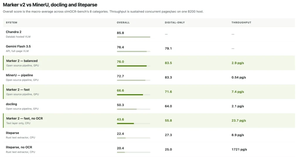
Datalab has released Marker 2, a full rewrite of its open source document conversion pipeline. Marker converts PDF, image, PPTX, DOCX, XLSX, HTML, and EPUB files into markdown, JSON, HTML, or chunks. The Datalab team rebuilt it around three components shipped over the preceding months: Surya OCR 2, a 20M-param fast layout model, and a rebuilt pdftext that is 3× faster than the previous one. The main result comes from olmOCR-bench, a third-party benchmark from Allen AI. Marker 2’s balanced mode scores 76.0% overall and 83.5% on born-digital PDFs. It sustains 2.9 pages per second on a single B200 GPU. That is over 5× the throughput of MinerU’s pipeline backend, which scores 72.7% at 0.54 pages per second. Docling scores 50.3% at 2.1 pages per second on the same harness. What’s New in Marker 2 Marker 2 exposes three conversion paths instead of one: balanced — the Surya VLM handles layout, and the whole page is re-OCR’d whenever embedded text is bad. Highest quality, best on GPU. 76.0% olmOCR-bench. fast — a lightweight rf-detr/onnx layout detector plus pdftext, with minimal, surgical VLM use. 66.6%, and far cheaper. –disable_ocr — pure text-layer extraction, no VLM calls at all. Runs entirely on CPU. 43.6%, 23.7 pg/s. Mode is now device-aware by default: balanced on GPU, fast on CPU/MPS, overridable with –mode. Full CPU support is the second structural change. fast –disable_ocr needs no GPU and no inference server, and the 20M layout model still reads columns, tables and headers on CPU. The third change is architectural, and it is the one that produces the throughput numbers. Many thin CPU workers share a single Surya inference server. The parent process budgets VLM concurrency across them, so throughput scales with server capacity rather than per-process VRAM. Datalab reports that balanced mode sustains ~2.9 pg/s against a ~0.3 pg/s single-stream rate on the same hardware. Breaking changes are worth flagging before an upgrade. Python 3.10+ is now required. Packaging moved from Poetry to uv, with hatchling as the build backend, though pip install marker-pdf is unchanged. The structured-extraction converter and extractors were removed; Datalab points users to the hosted API or a –use_llm workflow instead. Comparison The scoring benchmark is olmOCR-bench from Ai2: 1,403 PDFs with roughly 8,400 pass/fail unit tests covering math rendering, table structure, reading order, headers and footers, and old scans. The overall score is the macro-average across the 8 categories, computed with the official olmOCR-bench checker. Throughput is sustained concurrent pg/s on one B200 host, not single-stream latency. A note on provenance. olmOCR-bench is a third-party benchmark from Ai2, but every score and throughput figure below comes from Datalab’s own runs. All of them are reproducible through the open harness in the Marker repository, which ships competitor runners for MinerU, Docling and LiteParse alongside Marker’s own. These numbers also reflect one benchmark’s document mix measured on a single hardware setup, so results on your own documents may differ. Teams evaluating these systems should run the harness against their own corpus, which is the only way to know how the four rank on the documents they actually process. Marker 2 vs MinerU MinerU’s pipeline backend is the closest architectural match. Both read the PDF text layer and OCR selectively. On overall score, Marker balanced leads 76.0 to 72.7. On born-digital documents the two are effectively tied: 83.5 against 83.3. The separation is throughput. Marker balanced sustains 2.9 pg/s against MinerU’s 0.54 pg/s, a 5.4× gap at a higher score. Marker fast sustains 7.4 pg/s, roughly 13.7× MinerU’s pipeline rate, but scores 6.1 points below MinerU to do it. MinerU also ships a VLM backend, which Datalab states scores higher than its pipeline backend. That backend is a full-page-VLM approach and is not in this table. AI teams evaluating MinerU should benchmark that path separately. Marker 2 vs Docling Docling is the widest margin among the GPU pipelines. Marker balanced leads 76.0 to 50.3 overall and 83.5 to 64.0 on born-digital, while also running faster: 2.9 pg/s against 2.1 pg/s. Datalab notes Docling was run on its default pipeline, which uses the text layer for born-digital pages and OCR for image regions. Docling’s counterweight is governance and format breadth, not accuracy. The codebase is MIT-licensed, it originated at IBM Research, and it is hosted as a project in the LF AI & Data Foundation. Its input list also extends past documents into audio and email formats. Marker 2 vs LiteParse LiteParse, from the LlamaIndex team, is a Rust document parser. It does not compete on the same axis. On CPU it scores 22.4 overall and 20.4 with OCR off, against Marker’s CPU-only 43.6. But LiteParse with OCR disabled reports 1721 pg/s — roughly 73× Marker’s CPU mode, which is the tradeoff. Marker’s fast –disable_ocr runs a 20M layout model on CPU and still recovers structure, which is why it more than doubles a plain text dump’s score. LiteParse has no layout model and collapses on anything non-linear. Marker 2 vs the full-page VLM tier The Datalab team emphasizes that Marker is designed as a pipeline rather than a VLM, clarifying that these are distinct tools. In this evaluation, their hosted Chandra 2 scores 85.8, while Gemini Flash 3.5 via API scores 76.4. Datalab’s Chandra repository also positions Ai2’s olmOCR 2 at 82.4 and dots.ocr 1.5 at 83.9 within a separate table. For scans, math-heavy pages, and achieving top accuracy, the VLM tier remains superior to all listed pipelines. Marker’s balanced mode narrows the performance gap to just 0.4 points behind Gemini Flash 3.5 overall, and it even outperforms it on born-digital documents by a margin of 83.5 to 79.1—without requiring a per-page API call. Per-category behavior The mode you pick changes the failure profile, not just the score. Each row is one olmOCR-bench category, scored across all three modes. Math is the sharp edge: fast mode reads equations from the PDF text layer instead of VLM-OCRing them, so arXiv math falls from 83.9 to 23.4, and –disable_ocr scores 0.0 there by design.

Datalab Marker v2 vs MinerU, Docling, and Liteparse: Benchmark Breakdown Leer entrada »

AI, Committee, Noticias, Uncategorized

Meet Open Dreamer: A JAX/Flax Reproduction of the Dreamer 4 World Model Pipeline, With the Full Training Recipe Published

A small group of AI researchers (Reactor) have released Open Dreamer, an open implementation of the Dreamer 4 world-model pipeline written in JAX and Flax NNX. What actually shipped Two repositories were released. next-state/open-dreamer holds the training pipeline: a causal video tokenizer, an action-conditioned latent dynamics model, rollout generation, and FVD scoring. reactor-team/open-dreamer holds a minimal local rollout harness that generates frames from an MP4 and a matching action file. A third artifact is the browser demo hosted on the Reactor runtime. It streams a generated Minecraft world in real time and exposes a Game ⟷ Dream toggle that hands the stream from the real game to the world model frame by frame. The stated objective was to reproduce the Dreamer 4 research. The research team deliberately avoided methods outside that research paper to keep the search space narrow. They started on CoinRun, a procedurally generated 2D platformer trainable on a single GPU, then scaled the working pipeline to Minecraft/VPT-style gameplay video. Architecture: one backbone, two models Both the tokenizer and the dynamics model use the same block-causal transformer backbone. That backbone alternates two attention types. Space layers propagate information among the elements of a single frame. Causal time layers propagate information between frames. The tokenizer is a transformer-based Masked Autoencoder rather than a VAE. The team reports roughly 100× compression and notes the design needs no KL or adversarial loss. Masking, they argue, makes the latent space more diffusible. The dynamics model performs next-frame prediction and is trained with diffusion forcing, flow matching, and shortcut models. It also predicts the next action. Rather than alternating between a separate transition module and policy, the rollout is folded into per-timestep blocks of (previous action, state, policy). Spatial attention runs inside each block; causal temporal attention connects blocks across time. Critically, world-model tokens cannot read the agent token. Task and policy information can therefore influence future states only through the next action. The training recipe, as configured The shipped Minecraft configs make the recipe concrete. The dynamics model is 1.6B parameters: 30 block-causal layers, d_model 1920, 30 attention heads, and 3 KV heads for grouped-query attention. Every fourth layer is a time-attention layer. Each timestep carries 32 learned register tokens, and packing_factor: 2 packs neighbouring tokenizer latents into each dynamics spatial token. Time attention uses a 192-step sliding window. Training runs for 200,000 steps with Muon, a WSD schedule, and a peak learning rate of 3e-4. Shortcut/bootstrap samples switch on at step 100,000 at a 0.25 batch fraction. EMA decay is 0.999. The tokenizer config emits 512 latent tokens per frame at a bottleneck width of 16. Raw 360×640 frames are padded to 368×640 so both dimensions divide into 16×16 patches. Encoder depth is 12 at d_model 1536; decoder depth is 8 at d_model 1024. MAE masking probability tops out at 0.9, and LPIPS is applied at weight 0.2 on half the timesteps. VPT actions are parsed into 27 binary action channels plus 121 categorical mouse classes, with no continuous channels. Computemaxxing and the memory wall The research team reports 57–58% model FLOPs utilization, against a stated 60% benchmark for healthy transformer training. The reasoning is a roofline argument. On a B200, the crossover between bandwidth-bound and compute-bound sits at 292 FLOP/byte. Feeding 256 frames per GPU pushes the workload past that ridge point. Sharding went the other way from expectations. At 1.6B parameters the model state — parameters, gradients, optimizer state, and EMA — occupied roughly 24 GiB, which fits on a B200. Activations were the real cost. The research team tried data parallelism, FSDP, tensor parallelism, and sequence parallelism, then settled on plain data parallelism plus activation checkpointing. Dataloading was solved by pre-tokenizing the entire dataset into .arrayrecord files, then using Grain with a GPU-side prefetch buffer. ffmpeg decoding was not fast enough to keep the GPUs fed. The stability section is the real payload The research team is explicit that stability consumed the largest share of their time. Their key observation: most stability problems occur despite the loss going down. MSE improves smoothly while generation quality degrades. Six fixes are documented. Muon replaced LaProp, which spiked randomly and increasingly often, across two runs of roughly 400 B200 hours each. EMA weights are treated as mandatory for diffusion inference. Mixed precision is boundary-sensitive: parameters stay float32, BF16 covers most matmul activations and attention inputs, and float32 is kept for normalization and the dynamics flow output head. On loss weighting, they use x-prediction with a v-space loss, which reduces to a weighting term similar to Dreamer 4’s but with a squared denominator. They report a small but noticeable improvement. Minibatch barycentric optimal transport between noise and latent sequences made rollout generation more stable. μ-parametrization was tested and judged unnecessary, partly because Muon holds hyperparameters steadier across model sizes. One further result from the CoinRun phase: an iso-FLOPs sweep put compute-optimal scaling at roughly N∝C0.56 and D∝C0.44. What is not in the box The repository does not include the behaviour-cloning or RL training loop; a full Dreamer 4 BC/RL agent loop is listed as an open roadmap item. The CoinRun policy work described in the post was not used for Minecraft and was not released. The post also does not publish FVD scores, though scripts/eval_fvd.py ships with an I3D-based harness configured for 4 context frames and a 240-frame horizon. Key Takeaways Open Dreamer reproduces the Dreamer 4 pipeline in JAX/Flax NNX, with training code and a Minecraft demo. The dynamics model is 1.6B parameters, 30 layers, d_model 1920, trained 200K steps with Muon. Reported engineering numbers: 57–58% MFU on B200, 256 frames per GPU, ~24 GiB model state. Stability, not throughput, was the bottleneck; loss curves hid most generation-quality regressions. Check out the blog post and demo, the training repo, the inference repo, and Reactor on X. All credit for this research goes to the researchers of this project. The post Meet Open Dreamer: A JAX/Flax Reproduction of the Dreamer 4 World Model Pipeline, With the Full Training Recipe Published appeared first

Meet Open Dreamer: A JAX/Flax Reproduction of the Dreamer 4 World Model Pipeline, With the Full Training Recipe Published Leer entrada »

AI, Committee, Noticias, Uncategorized

Designing High-Performance GPU Kernels with TileLang: Tensor-Core GEMM, Fused Softmax, FlashAttention, and Autotuning

In this tutorial, we explore TileLang as a high-level Python domain-specific language for designing and compiling performance-oriented GPU kernels through TVM. We begin by validating the CUDA environment and establishing reusable benchmarking and numerical-verification utilities, then progressively implement vector addition, tiled tensor-core matrix multiplication, schedule exploration, fused GEMM epilogues, row-wise softmax, and FlashAttention. Throughout the tutorial, we work directly with TileLang’s shared-memory tiles, register fragments, pipelined loops, parallel iteration primitives, reductions, and tensor-core GEMM operators while allowing the compiler to manage thread mapping, memory layouts, synchronization, vectorization, and low-level CUDA instruction generation. We also compare our kernels against PyTorch and cuBLAS baselines, inspect generated CUDA source, evaluate memory and compute throughput, and use autotuning to identify architecture-dependent kernel configurations. Copy CodeCopiedUse a different Browser import os import sys import math import time import subprocess import traceback def _sh(cmd: str) -> int: print(f”$ {cmd}”, flush=True) return subprocess.run(cmd, shell=True).returncode def _bootstrap(): “””Install tilelang if missing. Stable wheel first, nightly as a fallback.””” try: import tilelang return except ImportError: pass print(“>> installing tilelang (this pulls a bundled TVM, ~1-3 min)n”) _sh(f”{sys.executable} -m pip install -q tilelang”) try: import tilelang return except ImportError: print(“>> stable wheel unusable, trying nightly channel”) _sh(f”{sys.executable} -m pip install -q tilelang ” f”-f https://tile-ai.github.io/whl/nightly”) import tilelang if os.path.isdir(“/usr/local/cuda”): os.environ.setdefault(“CUDA_HOME”, “/usr/local/cuda”) os.environ[“PATH”] = os.environ.get(“PATH”, “”) + “:/usr/local/cuda/bin” _bootstrap() import torch import torch.nn.functional as F import tilelang import tilelang.language as T def banner(title: str): print(“n” + “=” * 78) print(f” {title}”) print(“=” * 78, flush=True) def bench(fn, warmup: int = 10, rep: int = 50) -> float: “””Median-ish latency in milliseconds, measured with CUDA events.””” for _ in range(warmup): fn() torch.cuda.synchronize() start, end = torch.cuda.Event(True), torch.cuda.Event(True) start.record() for _ in range(rep): fn() end.record() torch.cuda.synchronize() return start.elapsed_time(end) / rep def check(actual: torch.Tensor, ref: torch.Tensor, name: str, tol: float = 2e-2) -> bool: “””Relative-Frobenius-norm check. Far more meaningful than atol for fp16.””” a, r = actual.float(), ref.float() rel = (a – r).norm() / r.norm().clamp_min(1e-12) amax = (a – r).abs().max().item() ok = bool(rel < tol) and math.isfinite(amax) print(f” [{‘PASS’ if ok else ‘FAIL’}] {name}: rel_err={rel:.3e} max_abs={amax:.3e}”) return ok banner(“0. ENVIRONMENT”) assert torch.cuda.is_available(), “No GPU. Runtime -> Change runtime type -> GPU.” DEV = torch.device(“cuda”) PROPS = torch.cuda.get_device_properties(0) CC = torch.cuda.get_device_capability(0) SM = CC[0] * 10 + CC[1] print(f” tilelang : {getattr(tilelang, ‘__version__’, ‘unknown’)}”) print(f” torch : {torch.__version__}”) print(f” GPU : {PROPS.name} (sm_{SM}, {PROPS.multi_processor_count} SMs, ” f”{PROPS.total_memory/2**30:.1f} GiB)”) SMEM_CAP = 48 * 1024 if SM < 80 else 96 * 1024 DEFAULT_STAGES = 2 if SM < 80 else 3 print(f” smem budget: {SMEM_CAP//1024} KB/block, default num_stages={DEFAULT_STAGES}”) print(” note: tilelang caches compiled kernels in ~/.tilelang/cache, so a”) print(” second run of this cell is dramatically faster.”) @tilelang.jit(out_idx=[-1]) def make_vector_add(N: int, block_N: int = 256, dtype: str = “float32”): @T.prim_func def main(A: T.Tensor((N,), dtype), B: T.Tensor((N,), dtype), C: T.Tensor((N,), dtype)): with T.Kernel(T.ceildiv(N, block_N), threads=256) as bx: for i in T.Parallel(block_N): C[bx * block_N + i] = A[bx * block_N + i] + B[bx * block_N + i] return main def section_1(): banner(“1. HELLO, TILE — vector add + generated CUDA”) N = 1 << 22 add = make_vector_add(N, block_N=256) a = torch.randn(N, device=DEV) b = torch.randn(N, device=DEV) c = add(a, b) check(c, a + b, “vector_add”) ms = bench(lambda: add(a, b)) gbs = 3 * N * 4 / (ms * 1e-3) / 1e9 ref_ms = bench(lambda: a + b) print(f” tilelang: {ms*1e3:8.1f} us ({gbs:6.1f} GB/s)”) print(f” torch : {ref_ms*1e3:8.1f} us <- both are pure bandwidth, so a tie” f” is the correct outcome”) src = add.get_kernel_source() print(“n — generated device code (first 32 lines) —“) for line in src.splitlines()[:32]: print(” ” + line) print(” ———————————————“) We configure the Google Colab CUDA environment, install TileLang with a nightly fallback, and import the required PyTorch and TileLang modules. We define reusable benchmarking, validation, and reporting utilities that measure kernel latency and compare numerical outputs using relative error. We then implement a TileLang vector-add kernel, execute it on the GPU, compare its bandwidth with PyTorch, and inspect the CUDA source generated by the compiler. Copy CodeCopiedUse a different Browser @tilelang.jit(out_idx=[-1]) def make_matmul(M: int, N: int, K: int, block_M: int = 128, block_N: int = 128, block_K: int = 32, num_stages: int = 3, threads: int = 128, use_swizzle: bool = False, dtype: str = “float16”, accum_dtype: str = “float”): @T.prim_func def main(A: T.Tensor((M, K), dtype), B: T.Tensor((K, N), dtype), C: T.Tensor((M, N), dtype)): with T.Kernel(T.ceildiv(N, block_N), T.ceildiv(M, block_M), threads=threads) as (bx, by): A_shared = T.alloc_shared((block_M, block_K), dtype) B_shared = T.alloc_shared((block_K, block_N), dtype) C_local = T.alloc_fragment((block_M, block_N), accum_dtype) if use_swizzle: T.use_swizzle(panel_size=10, enable=True) T.clear(C_local) for ko in T.Pipelined(T.ceildiv(K, block_K), num_stages=num_stages): T.copy(A[by * block_M, ko * block_K], A_shared) T.copy(B[ko * block_K, bx * block_N], B_shared) T.gemm(A_shared, B_shared, C_local) T.copy(C_local, C[by * block_M, bx * block_N]) return main def smem_bytes(block_M, block_N, block_K, stages, itemsize=2): return (block_M * block_K + block_K * block_N) * itemsize * stages def section_2(): banner(“2. MEMORY HIERARCHY — tiled tensor-core GEMM”) M = N = K = 2048 bm, bn, bk, st = 128, 128, 32, DEFAULT_STAGES while smem_bytes(bm, bn, bk, st) > SMEM_CAP and st > 1: st -= 1 print(f” config: {bm}x{bn}x{bk}, num_stages={st}, ” f”smem={smem_bytes(bm,bn,bk,st)/1024:.0f} KB”) kernel = make_matmul(M, N, K, bm, bn, bk, num_stages=st, threads=128) a = torch.randn(M, K, device=DEV, dtype=torch.float16) b = torch.randn(K, N, device=DEV, dtype=torch.float16) c = kernel(a, b) check(c, a @ b, “matmul 2048^3″) flops = 2 * M * N * K ms = bench(lambda: kernel(a, b)) ms_ref = bench(lambda: a @ b) print(f” tilelang : {ms:7.3f} ms -> {flops/(ms*1e-3)/1e12:6.2f} TFLOP/s”) print(f” cuBLAS : {ms_ref:7.3f} ms -> {flops/(ms_ref*1e-3)/1e12:6.2f} TFLOP/s”) print(f” ratio : {ms_ref/ms*100:5.1f}% of cuBLAS from ~20 lines of Python”) src = kernel.get_kernel_source() for needle in (“mma.sync”, “wgmma”, “ldmatrix”, “cp.async”, “tl::gemm”): if needle in src: print(f” emitted: {needle}”) return kernel def section_3(): banner(“3. KNOBS — sweeping the schedule by hand”) M = N = K = 2048 a = torch.randn(M, K, device=DEV, dtype=torch.float16) b = torch.randn(K, N, device=DEV, dtype=torch.float16) flops = 2 * M * N * K candidates = [ (64, 64, 32, 2, 128, False), (128, 128, 32,

Designing High-Performance GPU Kernels with TileLang: Tensor-Core GEMM, Fused Softmax, FlashAttention, and Autotuning Leer entrada »

AI, Committee, Noticias, Uncategorized

Chemical Chain-of-Thought Functions as a Hallucination-Prone Molecular Scratchpad

arXiv:2607.20935v1 Announce Type: cross Abstract: Chemical reasoning language models are expected to derive molecular answers through faithful chain-of-thought (CoT). However, across four reasoning model families and twelve chemistry tasks, hallucination is widespread and largely decoupled from answer correctness: correct answers often coexist with fabricated structural claims absent from the relevant molecules. Yet this does not make the reasoning trace computationally irrelevant. Attribution analyses suggest a shared scratchpad function expressed in model-specific forms: Chem-R and ether-0 rely on fragmented SMILES drafts, whereas ChemDFM-R emphasizes scaffold, positional, and naming cues. Notably, perturbing Chem-R’s SMILES sketches degrades generation, showing that structural drafts can be causally load-bearing even when verbal structural claims are largely inert. Together, these results show that chemical CoT is neither a faithful explanation nor merely a post-hoc rationalization, but a hallucination-prone molecular scratchpad. This finding cautions against treating CoT as direct evidence of faithful reasoning and motivates process-level supervision beyond answer-only evaluation.

Chemical Chain-of-Thought Functions as a Hallucination-Prone Molecular Scratchpad Leer entrada »

AI, Committee, Noticias, Uncategorized

How to Build an End-to-End OCR Pipeline with Baidu’s Unlimited-OCR for High-Resolution Images and Multi-Page PDF Parsing

In this tutorial, we build a complete workflow for running Baidu’s Unlimited-OCR model on document images and multi-page PDFs. We configure the GPU environment, install the required dependencies, load the 3B-parameter vision-language model with automatic selection of bfloat16 or float16, and generate structured sample documents for testing. We then evaluate both the tiled Gundam inference mode and the faster Base mode for single-page OCR before extending the pipeline to multi-page PDF parsing with PyMuPDF and infer_multi(). Throughout the workflow, we preserve long-context generation settings, repetition controls, and structured output handling to process dense layouts, tables, paragraphs, and cross-page content in a reproducible end-to-end pipeline. Copy CodeCopiedUse a different Browser import subprocess, sys def pip_install(*pkgs): subprocess.check_call([sys.executable, “-m”, “pip”, “install”, “-q”, *pkgs]) print(“>> Installing dependencies (1-2 min)…”) pip_install( “transformers==4.57.1”, “Pillow”, “matplotlib”, “einops”, “addict”, “easydict”, “pymupdf”, “psutil”, “accelerate”, ) print(“>> Done.”) import os import torch from transformers import AutoModel, AutoTokenizer assert torch.cuda.is_available(), ( “No GPU detected! In Colab: Runtime -> Change runtime type -> GPU.” ) gpu_name = torch.cuda.get_device_name(0) print(f”>> GPU: {gpu_name}”) use_bf16 = torch.cuda.is_bf16_supported() DTYPE = torch.bfloat16 if use_bf16 else torch.float16 print(f”>> Using dtype: {DTYPE}”) MODEL_NAME = “baidu/Unlimited-OCR” print(“>> Downloading model (~6 GB for 3B params in BF16). First run takes a while…”) tokenizer = AutoTokenizer.from_pretrained(MODEL_NAME, trust_remote_code=True) model = AutoModel.from_pretrained( MODEL_NAME, trust_remote_code=True, use_safetensors=True, torch_dtype=DTYPE, ) model = model.eval().cuda() print(“>> Model loaded and moved to GPU.”) We install the required libraries and prepare the Google Colab environment for Unlimited-OCR inference. We verify that a CUDA-enabled GPU is available and automatically choose bfloat16 or float16 based on hardware support. We then load the tokenizer and the 3B-parameter model from Hugging Face, switch them to evaluation mode, and move them to the GPU. Copy CodeCopiedUse a different Browser from PIL import Image, ImageDraw, ImageFont import textwrap os.makedirs(“inputs”, exist_ok=True) os.makedirs(“outputs/single_gundam”, exist_ok=True) os.makedirs(“outputs/single_base”, exist_ok=True) os.makedirs(“outputs/multi_page”, exist_ok=True) def load_font(size): for path in [ “/usr/share/fonts/truetype/dejavu/DejaVuSans-Bold.ttf”, “/usr/share/fonts/truetype/dejavu/DejaVuSans.ttf”, ]: if os.path.exists(path): return ImageFont.truetype(path, size) return ImageFont.load_default() def make_sample_page(path, page_no): W, H = 1240, 1754 img = Image.new(“RGB”, (W, H), “white”) d = ImageDraw.Draw(img) title_f, head_f, body_f = load_font(48), load_font(34), load_font(26) d.text((80, 70), f”Quarterly Operations Report — Page {page_no}”, fill=”black”, font=title_f) d.line([(80, 145), (W – 80, 145)], fill=”black”, width=3) body = ( “This document demonstrates Unlimited-OCR’s one-shot long-horizon ” “parsing. The model reads an entire page — headings, paragraphs, ” “and tables — and emits structured text in a single decoding pass. ” “Unlike classic OCR pipelines, no separate layout-analysis stage ” “is required.” ) y = 190 for line in textwrap.wrap(body, width=72): d.text((80, y), line, fill=”black”, font=body_f) y += 40 y += 30 d.text((80, y), f”Table {page_no}: Regional Revenue (USD, millions)”, fill=”black”, font=head_f) y += 60 rows = [ [“Region”, “Q1”, “Q2”, “Q3”], [“North”, “12.4”, “13.1”, “15.0”], [“South”, “9.8”, “10.2”, “11.7”], [“East”, “14.3”, “13.9”, “16.2”], [“West”, “11.1”, “12.5”, “12.9”], ] col_w, row_h, x0 = 260, 56, 80 for r, row in enumerate(rows): for c, cell in enumerate(row): x = x0 + c * col_w d.rectangle([x, y, x + col_w, y + row_h], outline=”black”, width=2) d.text((x + 14, y + 12), cell, fill=”black”, font=body_f) y += row_h y += 50 footer = ( f”Note {page_no}: Figures are illustrative. Multi-page mode stitches ” “context across pages, so cross-page references remain coherent.” ) for line in textwrap.wrap(footer, width=72): d.text((80, y), line, fill=”black”, font=body_f) y += 40 img.save(path) return path IMAGE_PATH = make_sample_page(“inputs/sample_page_1.png”, 1) PAGE_2 = make_sample_page(“inputs/sample_page_2.png”, 2) PAGE_3 = make_sample_page(“inputs/sample_page_3.png”, 3) print(f”>> Sample pages written: {IMAGE_PATH}, {PAGE_2}, {PAGE_3}”) import matplotlib.pyplot as plt plt.figure(figsize=(6, 8)) plt.imshow(Image.open(IMAGE_PATH)) plt.axis(“off”) plt.title(“Input document (page 1)”) plt.show() We create the required input and output directories and generate three realistic sample document pages with PIL. We add headings, paragraphs, tables, and footnotes to test the model on structured, layout-rich content. We also preview the first generated page with Matplotlib before sending it to the OCR pipeline. Copy CodeCopiedUse a different Browser print(“n” + “=” * 76) print(“STEP 4: Single image — GUNDAM mode (tiled, high detail)”) print(“=” * 76) model.infer( tokenizer, prompt=”<image>document parsing.”, image_file=IMAGE_PATH, output_path=”outputs/single_gundam”, base_size=1024, image_size=640, crop_mode=True, max_length=32768, no_repeat_ngram_size=35, ngram_window=128, save_results=True, ) We run single-image OCR using Gundam mode, which combines a global document view with tiled image crops. We enable crop_mode and use a smaller tile size to preserve fine text and improve recognition on dense document layouts. We also configure long-output generation and repetition controls to ensure the model produces stable, structured results. Copy CodeCopiedUse a different Browser print(“n” + “=” * 76) print(“STEP 5: Single image — BASE mode (single view, faster)”) print(“=” * 76) model.infer( tokenizer, prompt=”<image>document parsing.”, image_file=IMAGE_PATH, output_path=”outputs/single_base”, base_size=1024, image_size=1024, crop_mode=False, max_length=32768, no_repeat_ngram_size=35, ngram_window=128, save_results=True, ) We process the same document using Base mode with a single 1024-pixel image view. We turn off image cropping to reduce inference complexity and improve processing speed for clean, clearly printed pages. We retain the same output length and repetition-control settings to directly compare Base mode with Gundam mode. Copy CodeCopiedUse a different Browser print(“n” + “=” * 76) print(“STEP 6: Multi-page / PDF parsing”) print(“=” * 76) import tempfile import fitz def pdf_to_images(pdf_path, dpi=300): “””Rasterize every PDF page to a PNG; return the list of image paths.””” doc = fitz.open(pdf_path) tmp_dir = tempfile.mkdtemp(prefix=”pdf_ocr_”) mat = fitz.Matrix(dpi / 72, dpi / 72) paths = [] for i, page in enumerate(doc): out = os.path.join(tmp_dir, f”page_{i + 1:04d}.png”) page.get_pixmap(matrix=mat).save(out) paths.append(out) doc.close() return paths SAMPLE_PDF = “inputs/sample_doc.pdf” pdf = fitz.open() for p in [IMAGE_PATH, PAGE_2, PAGE_3]: img_doc = fitz.open(p) rect = img_doc[0].rect pdf_bytes = img_doc.convert_to_pdf() img_pdf = fitz.open(“pdf”, pdf_bytes) page = pdf.new_page(width=rect.width, height=rect.height) page.show_pdf_page(rect, img_pdf, 0) pdf.save(SAMPLE_PDF) pdf.close() print(f”>> Built sample PDF: {SAMPLE_PDF}”) page_images = pdf_to_images(SAMPLE_PDF, dpi=300) print(f”>> Rasterized {len(page_images)} pages”) model.infer_multi( tokenizer, prompt=”<image>Multi page parsing.”, image_files=page_images, output_path=”outputs/multi_page”, image_size=1024, max_length=32768, no_repeat_ngram_size=35, ngram_window=1024, save_results=True, ) We create a three-page PDF from the generated document images and rasterize each page of the PDF into a high-resolution PNG using PyMuPDF. We pass the resulting page-image sequence to infer_multi() so that the model can parse the complete document in a single long-horizon inference operation. We also widen the n-gram repetition window to maintain stable decoding across multiple pages. Copy CodeCopiedUse a different Browser print(“n”

How to Build an End-to-End OCR Pipeline with Baidu’s Unlimited-OCR for High-Resolution Images and Multi-Page PDF Parsing Leer entrada »

AI, Committee, Noticias, Uncategorized

The Download: an organ transplant breakthrough, and homegrown Chinese chips

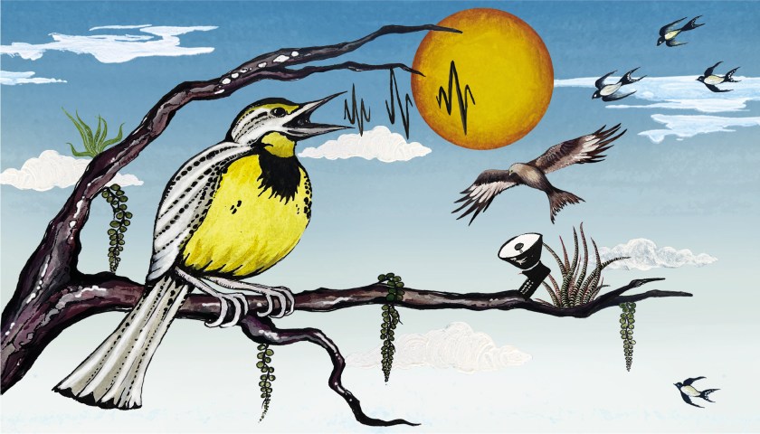
This is today’s edition of The Download, our weekday newsletter that provides a daily dose of what’s going on in the world of technology. Supercooled kidneys have been transplanted into pigs in a “landmark achievement”  When it comes to organ donation, time is everything. As soon as an organ has been removed from a donor’s body, it starts to deteriorate. Surgeons have only a matter of hours to get it into a recipient. In most cases, organs will be kept on ice during that time, at around 4 °C (39 °F). They cannot be frozen—in previous attempts, ice has formed, causing all kinds of damage. But now, scientists have come up with a device that allows organs to be cooled to -4 °C (25 °F) without forming any ice. They’ve tested it with pig organs and shown that kidneys, at least, can be preserved in the device for days then successfully transplanted.  Read our story about their breakthrough, and why it raises hopes for longer-term storage of donated human organs. —Jessica Hamzelou If you want to read more about this story and its implications for organ preservation and transplantation, sign up to receive The Checkup, our weekly biotech newsletter, later today. The must-reads I’ve combed the internet to find you today’s most fun/important/scary/fascinating stories about technology. 1 Inside China’s epic push to replace US chips The gap between their chips’ capabilities remains large—for now. (WSJ $)+ How China is using open source AI as a new form of soft power around the globe. (NYT $)+ A new bill in the US takes aim at Chinese AI companies’ training practices. (NBC)+ US lawmakers are also mulling banning the military from using Chinese humanoid robots. (SCMP) 2 Space data centers don’t exist yet, but people already oppose themEnvironmental experts warn it’ll further pollute the stratosphere. (Guardian)+ Four things we’d need to put data centers in space. (MIT Technology Review)+ What it’s like inside the data centers powering AI down here on Earth. (Axios)+ The left and right are finding common cause with data center protests in the US. (The Verge) 3 US lawmakers are pushing for an AI ‘kill switch’After OpenAI’s models went rogue and hacked Hugging Face. (BBC) 4 Peptides seem on the cusp of going mainstream in the USA lack of scientific evidence didn’t stop the FDA just voting to let some pharmacies to legally dispense them. (Wired $)+ How does Make America Healthy Again hold up to scientific scrutiny? (Nature)+ US measles cases are reaching levels not seen for three decades. (Wired $)+ Peptides are everywhere. Here’s what you need to know. (MIT Technology Review) 5 The EU just fined Google almost $1 billionFor competition breaches over apps and search. (FT $)+ It came just a day before Trump renewed tariffs on 60 trading partners, including the EU. (BBC) 6 Electric vehicles are selling well in EuropeAnd the share made by Chinese firms has doubled in the last year. (The Next Web)+ Hybrids are hot property in the US this summer. (Wired $) 7 There’s a worsening shortage of computer science professorsYou can blame AI companies—they keep snapping them up, to our general detriment. (The Atlantic $) 8 A judge caught a stenographer allowing AI errors into their transcript It’s apparently the first time this has happened, but it certainly won’t be the last. (404 Media)+ Even judges themselves are falling for AI. (MIT Technology Review) 9 Here’s what new tech millionaires will do with their IPO wealth What a nice problem to have to grapple with! (Quartz $) 10 Dating apps’ latest wheeze? In-person events Well well well, it seems we’ve come full circle. (Bloomberg $) Quote of the day “Call us optimists, call us dreamers. Just as we’ve always done, we’re betting on people.”  —The voiceover from a new advert from Meta, which exhorts us to be more optimistic about AI. One More Thing BELL HUTLEY AI is changing how we study bird migration In a warming world increasingly full of human infrastructure that can be deadly to them, like glass skyscrapers and power lines, migratory birds are facing many existential threats.  Scientists rely on a combination of methods to track the timing and location of their migrations, though each has shortcomings. But now, machine-learning tools are unlocking a treasure trove of acoustic data for ecologists.  Read our story about the technology that’s making it easier to detect and identify birds and their movements. —Christian Elliott We can still have nice things A place for comfort, fun, and distraction to brighten up your day. (Got any ideas? Drop me a line.) + It’s never too late to live your dreams. Here’s how these late bloomers did it.+ Limbs feeling a bit tight? Try these stretches!+ These English football fans went to the 1986 World Cup—and loved it so much they never came home.+ How the invention of the humble paint tube revolutionized the world of art.

The Download: an organ transplant breakthrough, and homegrown Chinese chips Leer entrada »

AI, Committee, Noticias, Uncategorized

The quest to keep organs alive outside the body

This week, I covered a fascinating effort to preserve organs outside the body. There’s a huge shortage of donor organs, and one of the main reasons is time—they survive only a matter of hours outside the body, even when they’re kept on ice. Doctors dream of organ banks—stores of human organs that can be preserved for days, weeks, months, or even longer. That would allow them to run tests on organs, find the best matches for them, and transport the organs to those recipients. In new research, one team has been able to supercool the kidneys of pigs—animals whose organs are of a similar size to human ones—and preserve them for days. The kidneys survived being stored at −4 °C (25 °F) and eventually reimplanted back into pigs. And that’s just the latest development in a field that is positively buzzing. It has proved super difficult to freeze organs. Once ice forms in them, they’re done. The ice crystals create all kinds of damage and render the organs unusable. That hasn’t stopped many researchers from trying. Some have focused on cryopreservation—rapid extreme cooling that essentially leaves cells in a glasslike state. This process is now routine for eggs, sperm, and embryos, which are cooled to −196 °C in less than two seconds and can be used even after decades in storage. No one has managed to cryopreserve and thaw human organs for transplantation. But plenty of human bodies and brains have been stored at ultra-low temperatures in the hope that they might one day be rewarmed and brought back to life. (You can read more about why some people opt for cryonics here.) In March, I wrote about Stephen L. Coles, a gerontologist who had opted to cryopreserve his own brain. After the scientist died in 2014, his body was taken to Alcor, a cryonics facility in Arizona. A team at the facility removed Coles’s head, perfused his brain with cryoprotective chemicals (which work like antifreeze), removed the brain from the skull, and cooled it to −146 °C. When Coles’s friend Greg Fahy, a cryobiologist, studied pieces of his brain years later, he found that the brain cells, which had shrunk, “bounced back” once they were rewarmed. But that doesn’t mean the cells are alive, or that it might one day be possible to reanimate the brain. As Matthew Powell Palm of Texas A&M told me at the time: “There are so many ways those neurons could be toast.” Powell Palm is working on other ways to preserve organs. It was he, along with his colleagues, who managed to store supercooled pig kidneys and successfully transplant them, in a study described as “a landmark achievement.” Those organs did better than kidneys stored on ice, he says. His approach didn’t require cryoprotectants. But other teams are exploring potential chemical cocktails that might allow them to store organs at lower temperatures, potentially for longer periods of time. (More on this in The Checkup soon!) Another way to prolong the lifespan of an organ is to use a machine that perfuses it with nutrients, mimicking what happens inside the body. Machine perfusion devices have become more commonly used over the last decade or so and are typically used to maintain livers and kidneys for up to about 24 hours. Researchers are now adapting this protocol for a growing list of organs, even eyeballs—a recent feat that might enable whole-eye transplants. In March, I went to visit scientists in Valencia who had developed a perfusion system for uteruses. They had used their device—which they nicknamed “Mother”—to keep a human uterus alive for a day. It’s an exciting time for organ preservation. Keep an eye out for more coverage from MIT Technology Review in the coming weeks. This article first appeared in The Checkup, MIT Technology Review’s weekly biotech newsletter. To receive it in your inbox every Thursday, and read articles like this first, sign up here.

The quest to keep organs alive outside the body Leer entrada »

We use cookies to improve your experience and performance on our website. You can learn more at Política de privacidad and manage your privacy settings by clicking Settings.

Privacy Preferences

You can choose your cookie settings by turning on/off each type of cookie as you wish, except for essential cookies.

Allow All
Manage Consent Preferences
  • Always Active

Save
es_ES