YouZum

AI

AI, Committee, Notizie, Uncategorized

Sakana AI Releases Fugu-Cyber: An Orchestration Model Reporting 86.9% on CyberGym and 72.1% on CTI-REALM

Sakana AI has released Fugu-Cyber (model ID is fugu-cyber-v1.0), a cybersecurity-specialized addition to its Fugu orchestration family. It is not just a new frontier model. It is a third endpoint on the Fugu orchestrator, tuned for security reasoning. Sakana launched that orchestrator a month earlier. Sakana reports a success rate of 86.9% on CyberGym and 72.1% on CTI-REALM. It describes those results as comparable to cyber-focused frontier models such as GPT-5.5-Cyber and Claude Mythos Preview. What the two benchmarks actually measure The two evaluations sit at opposite ends of a security workflow: CyberGym is a UC Berkeley benchmark of 1,507 real-world vulnerabilities across 188 OSS-Fuzz projects. In its main task, an agent receives a vulnerability description and an unpatched codebase. It must write a proof-of-concept that crashes the pre-patch build but not the post-patch build. That verification step is what makes the benchmark hard to game. CTI-REALM is Microsoft’s open-source detection-engineering benchmark. Microsoft curated 37 public threat reports from sources including Datadog Security Labs, Palo Alto Networks, and Splunk. An agent must map MITRE ATT&CK techniques, explore telemetry, iterate on KQL queries, and emit validated Sigma rules. Scoring covers Linux endpoints, Azure Kubernetes Service, and Azure cloud. Together the pair spans ‘find and prove the bug’ and ‘turn intel into a detection.’ That framing is the most defensible part of Sakana’s announcement. Where 86.9% sits against the field Context matters more than the number. When the CyberGym researchers published their first results, the best agent-model pairing reached roughly 20%. Anthropic reported 83.1% for Claude Mythos Preview under Project Glasswing in April 2026. OpenAI reported 85.6% for its updated GPT-5.5-Cyber, against 81.8% for GPT-5.5. Sakana’s 86.9% is therefore a small step past the reported frontier, not a jump. CTI-REALM is a different story. Microsoft’s own evaluation put the top three configurations, all Claude, in a band from 0.624 to 0.685. Fugu-Cyber’s 72.1% would sit above that band. One caveat matters. CTI-REALM is scored as a trajectory reward between 0 and 1. It is not a pass/fail rate. Sakana calls it a success rate anyway. How the orchestration works Fugu is itself a language model. It is trained to read a query and build an agentic scaffold on the fly. It then delegates sub-tasks to specialist models in a pool. The approach is documented in the Fugu technical report and two ICLR 2026 papers, TRINITY and the Conductor. TRINITY assigns Thinker, Worker, and Verifier roles across multiple LLMs. The Conductor learns natural-language coordination strategies through reinforcement learning. For security work, Sakana research team argues the verifier role is the point. A candidate vulnerability surfaced by one agent gets validated by security-specialized sub-agents before any patch is proposed. Routing remains proprietary, so you cannot see which model handled which step. Access, policy, and price Fugu-Cyber is gated on four dimensions. Access requires an application form stating the intended use case and verified contact details. Sakana team reviews each one manually. The model ships under an updated Acceptable Usage Policy that prohibits offensive misuse. Billing is restricted to the Token Plan. The $20, $100, and $200 subscription tiers cover Fugu and Fugu-Ultra only. And the Fugu API is not offered in the EU or EEA while Sakana works toward GDPR compliance. Pricing is fixed at $6 per million input tokens, $36 output, and $0.60 cached input. All three rates double above a 272K-token context. Every line is exactly 1.2× the Fugu-Ultra rate, a flat 20% premium for the cyber endpoint. Long codebase runs cross 272K easily, so the doubled tier is not an edge case. Key Takeaways Fugu-Cyber is an orchestration endpoint, not a new frontier model, launched July 21, 2026. Sakana reports 86.9% on CyberGym and 72.1% on CTI-REALM, both self-reported and un-replicated. Those scores edge past GPT-5.5-Cyber’s 85.6% and Claude Mythos Preview’s 83.1% on CyberGym. Access is gated: manual approval, defensive-use AUP, Token Plan only, no EU/EEA, no weights. Sakana’s own position is that a capable API along with human security expertise beats the API alone. The post Sakana AI Releases Fugu-Cyber: An Orchestration Model Reporting 86.9% on CyberGym and 72.1% on CTI-REALM appeared first on MarkTechPost.

Sakana AI Releases Fugu-Cyber: An Orchestration Model Reporting 86.9% on CyberGym and 72.1% on CTI-REALM Leggi l'articolo »

AI, Committee, Notizie, Uncategorized

Induction Labs Photon-1 Simulates Desktops, Plays Checkers, and Models Billiard Physics From One Pretraining Run

Most agents that learn from video need to know what action produced each frame. Induction Labs is arguing that this requirement is the bottleneck. Last week, they released imagination models, a foundation model architecture that pretrains on raw video with no action labels at all. Their test system is Photon-1, a sparse 106B-A5B mixture-of-experts (MoE) transformer trained on 18 years of computer demonstration video. On an internal computer use benchmark, Induction Labs reports that Photon-1 beats Gemini 3.1 Flash-Lite while using far less pretraining compute and costing roughly 3× less to serve. What an imagination model actually does An imagination model predicts future frames autoregressively using a next-latent-token-prediction objective. It does not generate pixels during pretraining. Everything is modeled in a learned representation space. The claim that matters is this: predicting future states teaches the model to complete tasks, even though it never sees an action during pretraining. Induction Labs calls this an implicit policy. The model learns concepts of what a person is doing, rather than a label for each mouse click. The compression trick that makes it scale The architecture depends on a vision encoder that uses finite scalar quantization (FSQ). Each frame is compressed into 960 discrete tokens. Each token is an 8-dimensional vector. Each dimension takes one of five values: −1, −1/2, 0, 1/2, 1. That gives a codebook of 5⁸ possible codes. The resulting encoding is about 2.2 KB per frame. Induction Labs reports over 100× better compression than existing OCR and multimodal-model representations, while preserving text, layout and state changes. To hit that rate, Photon-1 uses a differential latent encoder. It encodes video frames as pairs, so the latents describe differences between frames rather than frame contents. Data and pretraining compute The corpus starts from an internal index of 2 billion publicly available videos. Filtering reduces that to roughly 2 million computer screen recordings. An internal keyframe detection model strips redundant frames. The final dataset is 575 million frames, sampled at 1 frame per second. That equals 552 billion tokens, or about 18 years of video. Photon-1 was pretrained from scratch for a single epoch. Training the 106B-A5B MoE at 32K context took approximately 30,000 H200 GPU-hours, or 4.4×10²² training FLOPs. The research team implemented training in PyTorch with custom fused kernels for the vision encoder and MoE layers, sustaining 40% end-to-end MFU. Those three figures are mutually consistent: 30,000 H200-hours at 40% MFU lands almost exactly on 4.3×10²². From imagination to action Induction Labs finetuned Photon-1 on fewer than 35,000 computer use trajectories to teach the action and instruction format. Special computer use tokens let the model emit actions. At inference, Photon-1 predicts the next frame’s state first, then outputs the action that gets there. Online reinforcement learning follows. Rollouts run in real time on virtual machines at scale, and outcomes are verified programmatically to produce reward. The Linux VMs run five desktop environments (LXQt, Xfce, MATE, GNOME and Plasma), each with a Google account for login-restricted web apps and an internal ChatGPT clone with no rate limits. The compute and cost comparison Model Pretraining compute Weighted inference cost / 1M tokens* Gemini 3.1 Flash-Lite 1.200 × 10²⁴ FLOPs $0.36 Photon-1 0.044 × 10²⁴ FLOPs $0.11 *Weighted at a 10:1 input-to-output token ratio, which Induction Labs says matches its computer use tests. Two caveats belong next to that table. First, the Gemini figure is Induction Labs’ own conservative estimate, assuming 8B active parameters and 25T pretraining tokens. Taken at face value the ratio is about 27×, not the 30× headline; Induction Labs states “at least 30×” on the basis that the true Gemini number is likely higher and the model was likely distilled. Second, the benchmark is internal and unreleased, so the result is not independently reproducible today. Photon-1’s own breakeven cost on Induction Labs’ hardware is $0.06 per 1M input tokens and $0.60 per 1M output tokens, with no speculative decoding. Does it generalize past the desktop? This is the more interesting test, because Photon-1 saw only computer use video. The research team finetuned it on domains absent from pretraining and compared against two baselines: a vision encoder baseline with the same architecture and size but no imagination pretraining, and an LLM baseline (Ling-flash-2.0 from Inclusion AI, pretrained on 20T tokens). On 20,000 tournament checkers games from the Open Checkers Archive 2.0, Photon-1 beat both baselines on world simulation and on move quality. On 10,000 synthetically generated billiard games simulated at 5 fps, it produced a mean absolute error of 0.47 against the ground-truth physics engine, versus 1.15 for the LLM baseline and 1.44 for the vision encoder baseline. Photon-1 also picked up human priors from the pretraining video. After RL, it learned to use the in-VM ChatGPT clone to draft artifacts and answer knowledge questions, steering the LLM the way a person would. Key Takeaways Photon-1 learns an implicit policy from 18 years of screen recordings with zero action labels, using next-latent-token prediction. FSQ compresses each frame to 960 tokens (~2.2 KB), a reported 100× gain over OCR and multimodal representations. Trained for ~30,000 H200 GPU-hours, it beats Gemini 3.1 Flash-Lite on an internal benchmark at ~27× less pretraining compute. Despite seeing only desktop video, it beats an LLM baseline at checkers and billiard physics after finetuning. No weights, no API, no license — this is a research result, not a deployable model. Check out the full technical writeup from Induction Labs and the announcement thread on X. All credit for this research goes to the researchers of this project. The post Induction Labs Photon-1 Simulates Desktops, Plays Checkers, and Models Billiard Physics From One Pretraining Run appeared first on MarkTechPost.

Induction Labs Photon-1 Simulates Desktops, Plays Checkers, and Models Billiard Physics From One Pretraining Run Leggi l'articolo »

AI, Committee, Notizie, Uncategorized

FAIRChem v2 UMA for Multidomain Atomistic Simulation across Molecules, Catalysts, Materials, Vibrations, and Molecular Dynamics

In this tutorial, we explore FAIRChem v2 and the UMA universal machine-learning interatomic potential as a unified framework for atomistic simulation across molecular chemistry, catalysis, and inorganic materials. We configure an environment, authenticate with Hugging Face to access the gated UMA model weights, and initialize task-specific calculators for the omol, oc20, and omat domains. We then apply the same pretrained potential to a broad set of computational chemistry workflows, including single-point energy and force prediction, molecular geometry optimization, spin-state comparison, reaction-energy estimation, vibrational analysis, surface adsorption, crystal-cell relaxation, equation-of-state fitting, molecular dynamics, and potential-energy surface scanning. Throughout the tutorial, we integrate FAIRChem with the Atomic Simulation Environment to manage atomic structures, optimizers, constraints, thermodynamic calculations, and trajectory analysis while using GPU acceleration whenever it is available. Copy CodeCopiedUse a different Browser import importlib.util, subprocess, sys, os def _pip(*pkgs): subprocess.check_call([sys.executable, “-m”, “pip”, “install”, “-q”, *pkgs]) if importlib.util.find_spec(“fairchem”) is None: print(“>> Installing fairchem-core, ase, and helpers (takes ~2-4 min)…”) _pip(“fairchem-core”, “ase”, “matplotlib”, “huggingface_hub”) print(“>> Installation done.”) else: print(“>> fairchem already installed.”) from huggingface_hub import login, whoami def hf_authenticate(): token = None try: from google.colab import userdata token = userdata.get(“HF_TOKEN”) except Exception: pass token = token or os.environ.get(“HF_TOKEN”) try: whoami() print(“>> Already authenticated with Hugging Face.”) return except Exception: pass if token is None: from getpass import getpass token = getpass(“Paste your Hugging Face access token: “).strip() login(token=token) print(“>> Hugging Face login OK.”) hf_authenticate() import numpy as np import torch import matplotlib.pyplot as plt from fairchem.core import pretrained_mlip, FAIRChemCalculator DEVICE = “cuda” if torch.cuda.is_available() else “cpu” print(f”>> Using device: {DEVICE}”) MODEL = “uma-s-1p2″ predictor = pretrained_mlip.get_predict_unit(MODEL, device=DEVICE) calc_mol = FAIRChemCalculator(predictor, task_name=”omol”) calc_cat = FAIRChemCalculator(predictor, task_name=”oc20″) calc_mat = FAIRChemCalculator(predictor, task_name=”omat”) print(f”>> Loaded {MODEL} with omol / oc20 / omat calculators.”) We install the required FAIRChem, ASE, visualization, and Hugging Face dependencies while ensuring the setup remains safe to rerun in Google Colab. We authenticate with Hugging Face to access the gated UMA model weights and automatically detect whether GPU acceleration is available. We then load the UMA predictor and create separate calculators for molecular, catalysis, and materials simulations. Copy CodeCopiedUse a different Browser from ase.build import molecule from ase import Atoms print(“n” + “=”*70) print(“SECTION 2: Single-point energetics of water (omol task)”) print(“=”*70) h2o = molecule(“H2O”) h2o.info.update({“charge”: 0, “spin”: 1}) h2o.calc = calc_mol E_h2o = h2o.get_potential_energy() F_h2o = h2o.get_forces() print(f”E(H2O) = {E_h2o:.4f} eV”) print(f”Max |force| = {np.abs(F_h2o).max():.4f} eV/A”) def atom_energy(symbol, spin): a = Atoms(symbol, positions=[[0, 0, 0]]) a.info.update({“charge”: 0, “spin”: spin}) a.calc = calc_mol return a.get_potential_energy() E_O = atom_energy(“O”, spin=3) E_H = atom_energy(“H”, spin=2) E_atomization = -(E_h2o – E_O – 2 * E_H) print(f”Atomization energy of H2O = {E_atomization:.3f} eV ” f”(experiment ~ 9.5 eV incl. ZPE effects)”) from ase.optimize import LBFGS print(“n” + “=”*70) print(“SECTION 3: Relaxing a deliberately distorted water molecule”) print(“=”*70) h2o_bad = molecule(“H2O”) h2o_bad.positions[1] += [0.25, -0.10, 0.05] h2o_bad.info.update({“charge”: 0, “spin”: 1}) h2o_bad.calc = calc_mol opt = LBFGS(h2o_bad, logfile=None) energies_opt = [] opt.attach(lambda: energies_opt.append(h2o_bad.get_potential_energy())) opt.run(fmax=0.01, steps=200) d_OH = h2o_bad.get_distance(0, 1) ang = h2o_bad.get_angle(1, 0, 2) print(f”Converged in {opt.get_number_of_steps()} steps”) print(f”O-H bond length = {d_OH:.3f} A (expt ~0.958 A)”) print(f”H-O-H angle = {ang:.1f} deg (expt ~104.5 deg)”) plt.figure(figsize=(5, 3.2)) plt.plot(energies_opt, “o-“) plt.xlabel(“Optimizer step”); plt.ylabel(“Energy (eV)”) plt.title(“H2O geometry optimization”); plt.tight_layout(); plt.show() We use the molecular UMA calculator to evaluate the energy, atomic forces, and atomization energy of a water molecule. We define isolated hydrogen and oxygen reference atoms with the correct spin multiplicities to construct the atomization-energy calculation. We then distort the water geometry, relax it with the LBFGS optimizer, and analyze the converged bond length, bond angle, and energy trajectory. Copy CodeCopiedUse a different Browser print(“n” + “=”*70) print(“SECTION 4: CH2 singlet-triplet gap (UMA is spin-aware!)”) print(“=”*70) singlet = molecule(“CH2_s1A1d”); singlet.info.update({“charge”: 0, “spin”: 1}) triplet = molecule(“CH2_s3B1d”); triplet.info.update({“charge”: 0, “spin”: 3}) singlet.calc = FAIRChemCalculator(predictor, task_name=”omol”) triplet.calc = FAIRChemCalculator(predictor, task_name=”omol”) gap = triplet.get_potential_energy() – singlet.get_potential_energy() print(f”E(triplet) – E(singlet) = {gap:.3f} eV ” f”(negative => triplet ground state; expt ~ -0.39 eV)”) print(“n” + “=”*70) print(“SECTION 5: Reaction energy of CH4 + 2 O2 -> CO2 + 2 H2O”) print(“=”*70) def relaxed_energy(name, spin=1): m = molecule(name) m.info.update({“charge”: 0, “spin”: spin}) m.calc = FAIRChemCalculator(predictor, task_name=”omol”) LBFGS(m, logfile=None).run(fmax=0.02, steps=200) return m.get_potential_energy() E = { “CH4”: relaxed_energy(“CH4”), “O2”: relaxed_energy(“O2”, spin=3), “CO2”: relaxed_energy(“CO2”), “H2O”: relaxed_energy(“H2O”), } dE_rxn = (E[“CO2”] + 2*E[“H2O”]) – (E[“CH4”] + 2*E[“O2″]) print(f”Delta E (electronic) = {dE_rxn:.2f} eV = {dE_rxn*96.485:.0f} kJ/mol”) print(“Experimental combustion enthalpy ~ -890 kJ/mol (ZPE/thermal not included here)”) from ase.vibrations import Vibrations print(“n” + “=”*70) print(“SECTION 6: Vibrational frequencies of relaxed H2O”) print(“=”*70) vib = Vibrations(h2o_bad, name=”vib_h2o”) vib.run() freqs = np.real(vib.get_frequencies()) real_modes = [f for f in freqs if f > 200] print(“Vibrational modes (cm^-1):”, “, “.join(f”{f:.0f}” for f in real_modes)) print(“Experimental H2O: 1595 (bend), 3657 (sym stretch), 3756 (asym stretch)”) print(f”Zero-point energy = {vib.get_zero_point_energy():.3f} eV”) vib.clean() We compare the singlet and triplet electronic states of methylene to calculate its spin-state energy gap. We relax methane, oxygen, carbon dioxide, and water before combining their predicted energies to estimate the electronic reaction energy of methane combustion. We also perform a finite-difference vibrational analysis of relaxed water to obtain its normal-mode frequencies and zero-point energy. Copy CodeCopiedUse a different Browser from ase.build import fcc100, add_adsorbate from ase.constraints import FixAtoms print(“n” + “=”*70) print(“SECTION 7: CO/Cu(100) relaxation + adsorption energy (oc20 task)”) print(“=”*70) slab = fcc100(“Cu”, size=(3, 3, 3), vacuum=8.0, periodic=True) slab.set_constraint(FixAtoms(mask=[a.tag > 1 for a in slab])) add_adsorbate(slab, molecule(“CO”), height=2.0, position=”bridge”) slab.calc = calc_cat opt = LBFGS(slab, logfile=None) opt.run(fmax=0.05, steps=300) E_slab_ads = slab.get_potential_energy() print(f”Relaxed CO/Cu(100) in {opt.get_number_of_steps()} steps, ” f”E = {E_slab_ads:.3f} eV”) clean = fcc100(“Cu”, size=(3, 3, 3), vacuum=8.0, periodic=True) clean.set_constraint(FixAtoms(mask=[a.tag > 1 for a in clean])) clean.calc = FAIRChemCalculator(predictor, task_name=”oc20″) LBFGS(clean, logfile=None).run(fmax=0.05, steps=300) E_clean = clean.get_potential_energy() co = molecule(“CO”); co.info.update({“charge”: 0, “spin”: 1}) co.calc = FAIRChemCalculator(predictor, task_name=”omol”) LBFGS(co, logfile=None).run(fmax=0.02, steps=100) E_co = co.get_potential_energy() E_ads = E_slab_ads – E_clean – E_co print(f”E(clean slab) = {E_clean:.3f} eV, E(CO gas) = {E_co:.3f} eV”) print(f”Adsorption energy (naive cycle) = {E_ads:.3f} eV”) print(“(oc20 uses its own DFT reference scheme; for publication-grade numbers”) print(” keep all species within a consistent task/reference framework.)”) We construct a periodic

FAIRChem v2 UMA for Multidomain Atomistic Simulation across Molecules, Catalysts, Materials, Vibrations, and Molecular Dynamics Leggi l'articolo »

AI, Committee, Notizie, Uncategorized

KwaiKAT Team Releases KAT-Coder-V2.5: An Agentic Coding Model Trained on 100,000+ Verifiable Repository Environments

The KwaiKAT Team at Kuaishou has introduced the KAT-Coder-V2.5. It is a coding model trained to operate inside real, executable repositories rather than emit single-turn code. The served model is available through StreamLake. An open-weight variant, KAT-Coder-V2.5-Dev, was released separately on Hugging Face under Apache-2.0. AutoBuilder: environments that actually run the intended tests The research frames a verifiable task as a triplet. It needs a precise task description, an executable repository environment, and a set of validation tests. A patch is correct only if it passes all of them. Tasks are mined from real pull requests and commits, following the SWE-bench lineage. The merged code change supplies a golden patch and the accompanying test change supplies a test patch. Raw issue text is discarded as a specification. Instead, descriptions are regenerated into three parts: a problem statement grounded in the golden patch, requirements derived from the test patch, and interface constraints inferred from both. A clarity check then drops anything ambiguous, incomplete, underspecified, or internally inconsistent. AutoBuilder handles the environment side. A build agent analyzes the repository and writes a configuration script that installs dependencies and runs tests from a clean checkout. A verification agent executes that script in an isolated sandbox. The acceptance rule is the interesting part. Verification does not read exit codes or grep log patterns. It parses structured test-framework output, and accepts an environment only when more than 90% of expected tests are collected and pass/fail outcomes reproduce across runs. Failures are fed back as structured information for iterative repair. Combining a preconfigured base environment, build-system templates, and a retrievable library of distilled build recipes raised the construction success rate from 16.5% to 57.2%. The result is over 100,000 verifiable environments spanning 12 languages. Git history, commit metadata, and other exploitable traces are stripped so agents cannot read the reference solution out of the repo. Data Scaling Flywheel: filtering on process Filtering trajectories by final test success is misleading. Some passing runs rely on hard-coding, mechanism bypassing, or test-oriented shortcuts. Some failing runs contain valuable search, localization, and repair behavior. KwaiKAT addresses both directions. For near misses, targeted process-level hints indicate what to inspect or verify without revealing the solution. That alone raises the pass rate of previously zero-pass tasks to roughly 20%. Because hinted trajectories contain information unavailable at inference, the verified patch is then fixed and a hint-free trajectory is regenerated from the original task context. Only samples that pass verification, show no hint leakage, and stay consistent with the patch are retained. For passing runs, rule-based gates remove invalid, unstable, or exploitative trajectories. A scoring stage then rates exploration, localization, pre-edit reasoning, specification fidelity, repository conventions, patch minimality, verification quality, recovery behavior, and honesty. A third mechanism targets harness overfitting. Tool names, argument conventions, output formats, and prompt templates are randomized while functionality is preserved. Because verification is anchored to test outcomes rather than harness traces, one task can be re-served under many harness configurations. Realistic perturbations are injected too: missing dependencies, transient command failures, truncated outputs, and noisy logs. Explore the pipeline and the numbers Infrastructure failures capped rewards before algorithmic limits During KAT-Coder-V2 training, slow reward curves were initially blamed on the RL algorithm. However, an audit revealed that ~16% of trajectories failed due to sandbox infrastructure issues rather than the model policy, with boundary misalignments sometimes emptying observations for ~40 steps and corrupting rewards. Three infrastructure fixes followed. First, an early-release image eviction policy lowered disk usage from 95% to 60%, reducing timeout-induced invalid rollouts from 6–7% to under 1%. Second, correcting environment variables during remote sandbox initialization stopped system overrides that flipped rewards on 6–7% of samples, cutting errors below 1%. Third, the Gateway Server bypassed mainstream chat endpoints—which caused 40% token drift at a ~200-turn scale by re-applying apply_chat_template and re-tokenizing—and called /generate directly to ensure rollout token alignment. Together, these updates reduced the sandbox feedback error rate from roughly 16% to below 2% and cut training collapses by an order of magnitude. Asymmetric PPO and a three-tier reward The research team chose PPO with GAE over critic-free trajectory methods because production harnesses split sessions into structurally distinct samples, complicating group baselines. Using asymmetric actor–critic, the Critic gets privileged training context (rewards, tests, coverage, patches, metadata, future turns), while the Actor sees only rollout state. The Critic and extra context are discarded at inference. Rewards are three-tiered: Core Task Scores require all fail_to_pass and pass_to_pass tests to pass; Standard Behavior Constraints penalize duplication, bad tool calls, and debug remnants; Failed Trajectory Incentives score file retrieval via F2 and give partial test credit. Five experts fuse via Multi-Teacher On-Policy Distillation using reverse KL, an off-policy start, and drift-aware truncation from Prune-OPD. Results Under a unified Claude Code harness, KAT-Coder-V2.5 leads its panel on PinchBench with 94.9, beating Opus 4.8 at 93.5. It places second on SWE-Bench Pro (65.2 vs 69.2) and the internal KAT Code Bench (53.1 vs 57.3). However, it lags on Terminal-Bench 2.1, placing last with 60.7 behind GLM-5.1 (61.8) and Opus 4.8 (84.6). On SciCode, it scores 50.3, matching GLM-5.2. Notably, the open-weight KAT-Coder-V2.5-Dev is a separate 35B-total / 3B-active MoE post-trained on Qwen3.6-35B-A3B using 127K SFT examples, then RL. Evaluated on a separate in-house protocol, its results are not comparable to the main flagship table. Key Takeaways KwaiKAT treats agentic coding as an infrastructure problem, not a model-scale problem. AutoBuilder lifted environment construction success from 16.5% to 57.2%, yielding 100,000+ verifiable environments across 12 languages. A sandbox audit found ~16% of RL trajectories failed because of the sandbox, not the policy; fixes cut that to below 2%. KAT-Coder-V2.5 tops PinchBench at 94.9 and ranks second on SWE-Bench Pro at 65.2, behind Opus 4.8. The open-weight KAT-Coder-V2.5-Dev is a separate 35B-A3B MoE under Apache-2.0, with its own benchmark numbers. Check out the Paper, the Model Weight on Hugging Face, and the Product Page. All credit for this research goes to the researchers of this project. The post KwaiKAT Team Releases KAT-Coder-V2.5: An Agentic Coding Model

KwaiKAT Team Releases KAT-Coder-V2.5: An Agentic Coding Model Trained on 100,000+ Verifiable Repository Environments Leggi l'articolo »

AI, Committee, Notizie, Uncategorized

Black Forest Labs Releases FLUX 3: A Multimodal Flow Model for Image, Video, Audio and Robot Action Prediction

Black Forest Labs (BFL) has released FLUX 3, a multimodal foundation model that learns from images, videos and audio inside a single architecture. It is also the first FLUX model to ship video, audio and action prediction from one set of weights. The Black Forest Labs (BFL) research team argues that no single modality gives a complete description of the world. Images capture spatial structure at one instant. Video restores time and exposes physical dynamics. Audio reveals causal relationships between mechanical events and sound. Each is treated as a lossy projection of the same underlying reality. Training on all of them at once means the modalities constrain each other. The sound has to match the impact. The motion has to obey the mass. The research team calls FLUX 3 its first model built entirely on that principle. The method underneath: Self-Flow FLUX 3 builds on Self-Flow, BFL’s method for aligning multimodal generation and understanding in one architecture. Self-Flow combines the flow matching objective with a self-supervised feature reconstruction objective. The reference implementation on GitHub is Apache-2.0 and uses SiT-XL/2 with per-token timestep conditioning. It trains with a 25% per-token mask ratio and self-distillation from an EMA teacher at layer 20 to a student at layer 8. That released checkpoint is an ImageNet 256×256 research model, not FLUX 3. BFL states that it ‘significantly scaled up compute and data resources’ on the same approach to train FLUX 3 across video, images and audio simultaneously. Self-Flow itself was introduced in March 2026, so it is not new to this launch. What is new is the scale. What FLUX 3 Video does FLUX 3 Video generates clips up to 20 seconds long in a single generation, with native audio. The supported modes cover text-to-video, image-to-video, video-to-video from a reference clip, keyframe-to-video for controlled transitions, and generative video-audio continuation from input video and audio. BFL also lists multilingual dialogue, agentic chaining of clips into multi-shot sequences, and strong typography generation with animated designs. The BFL team reports particular strength in human facial expressions and in associating sounds with physical events. Performance BFL team published preliminary human preference results. The setup was 10-second text-to-video clips at 720p with audio. FLUX 3 was preferred over Luma Ray 3.2 in 93% of comparisons and over Runway Gen-4.5 in 77%. Against Grok Imagine Video the figure is up to 69%, then Kling v3 Pro at 60%, Happy Horse v1 at 59% and Happy Horse 1.1 at 57%. Against Seedance 2.0 and Gemini Omni Flash the result is 52%, close to a coin flip. Interactive Explorer bfl@flux-3:~/real-world-models Early Access Commands >spec >bench >compute >action >mimic >rollout >selfflow Type a command below, or press ↑ / ↓ in the prompt to cycle history. Every figure is sourced from Black Forest Labs or mimic robotics. flux3 $ Enter a command enter Sources: bfl.ai/blog/flux-3 · bfl.ai/blog/flux-3-mimic · mimicrobotics.com · figures dated 23 Jul 2026 Built by Marktechpost

Black Forest Labs Releases FLUX 3: A Multimodal Flow Model for Image, Video, Audio and Robot Action Prediction Leggi l'articolo »

AI, Committee, Notizie, Uncategorized

Meet the New Claude Opus 5: Frontier-Class Agentic Coding and Computer Use at Unchanged Opus Pricing

Today, Anthropic released Claude Opus 5. It replaces Claude Opus 4.8 as the Opus-tier flagship. Pricing is unchanged at $5 per million input tokens and $25 per million output tokens. The Anthropic team positions Opus 5 as approaching the intelligence of Claude Fable 5 at half the price. It is now the default model on Claude Max and the strongest model on Claude Pro. What actually changed at the API level Three changes are quite important before any benchmark does: Thinking is on by default. On Opus 4.8, requests ran without thinking unless you set thinking: {“type”: “adaptive”}. On Opus 5 the same request thinks, and the effort parameter controls depth. Because max_tokens caps thinking plus response text, existing values need review. There is a breaking change. Setting thinking: {“type”: “disabled”} with effort xhigh or max now returns a 400 error. The restriction is enforced per request. You either cap effort at high or drop the thinking field. Anthropic tells developers to delete their verification prompts. Instructions like “include a final verification step” now cause over-verification, because the model already verifies its own work. The Opus 5 prompting guide covers the tuning patterns. The model ID is claude-opus-5. Context is 1M tokens as both default and maximum, with no smaller variant. Maximum output is 128k tokens on the synchronous Messages API. The Message Batches API reaches 300k with the output-300k-2026-03-24 beta header. The minimum cacheable prompt drops to 512 tokens, down from 1,024. Coding and agentic results On FrontierBench v0.1, a 74-task successor to Terminal-Bench 2.1, Opus 5 scored 43.3% at max effort. Opus 4.8 scored 18.7%. Fable 5 reached 33.7% and GPT-5.6 Sol reached 37.5%. At xhigh effort Opus 5 reaches 44.4% mean reward, its best result. One detail from that run is worth noting. Opus 5 safety classifiers flagged and refused 5% of API calls, across 4% of trials. Fable 5 classifiers flagged 42% of calls across 26% of trials. Opus 5 scored 96.0% on SWE-bench Verified and 79.2% on SWE-bench Pro. Fable 5 still edges it on Pro at 80.0%. On SWE-bench Multimodal the jump is larger, from 38.4% to 59.4%. The agentic numbers are the clearest wins. Opus 5 reached 70.57% on OSWorld 2.0 against 55.7% for Opus 4.8. On Zapier AutomationBench it scored 26.0%, against 17.0% for Opus 4.8 and 17.4% for Fable 5. At medium effort it still scores 24% at $0.89 per task. On Artificial Analysis GDPval-AA v2, Opus 5 takes the top two leaderboard spots at ELO 1861 and 1827. The xhigh setting beats every other model while using 25% fewer output tokens than max. Reasoning, and the ARC-AGI-3 result Anthropic prompted Opus 5 on all six IMO 2026 problems without tools or an agent harness. A three-model judge panel scored all 24 generated solutions correct. Human experts independently graded one pre-specified solution per problem at 7/7. The final 42/42 is gold-medal level, above the 29/42 cutoff. The ARC Prize Foundation reports a verified 30.16% on ARC-AGI-3 at high effort. That is roughly four times the best previously reported leaderboard score. GPT-5.6 Sol reached 7.78% and Opus 4.8 reached 1.52%. Opus 5 results at max effort were unavailable at release. On Humanity’s Last Exam, Opus 5 scored 56.3% without tools and 64.7% with them. Tools beat thinking on multimodal work The multimodal section carries a practical lesson. Agentic tool use scales test-time compute more cost-effectively than adaptive thinking alone. On Chartography, Opus 5 scored 29.6% without tools and 83.0% with a container and an image-cropping tool. On BenchCAD Vision2Code, voxel IoU moves from 0.366 to 0.821. With tools, that beats Claude Mythos 5 at 0.678 by a wide margin. Cyber capability rose, and safeguards were relaxed in one place Anthropic did not train Opus 5 on cybersecurity tasks. Capability rose anyway, as a byproduct of general capability gains. On ExploitBench, Opus 5 captured 10.14 mean capability flags in the AutoNudge arm. It produced 99 full arbitrary-code-execution exploits. Mythos 5 produced 132. On OSS-Fuzz, Opus 5 scored non-zero on 79.4% of targets. Mythos 5 reached roughly 80%. But Opus 5 completed 4 full exploits to Mythos 5’s 13. That gap defines the safeguard design. Opus 5 is nearly as strong as Mythos 5 at finding vulnerabilities, and substantially behind at exploiting them. So Anthropic unblocked vulnerability finding in source code. Binary-based scanning, penetration testing and exploit generation stay blocked. Classifiers are expected to intervene around 85% less often than on Fable 5. Defenders can apply to the Cyber Verification Program. UK AISI tested early checkpoints on three cyber ranges at 100M tokens per attempt. Opus 5 solved ‘The Last Ones’ end-to-end in 8 of 10 attempts. It did not solve the harder ‘Doing Life’ range. It reached step 22 of 23, further than any model tested. Under the RSP, Anthropic treats Opus 5 as having CB-1 capabilities but not CB-2. It applies the same ASL-3 protections used for Opus 4.8. The AI R&D threshold is not crossed. Prompt injection is the standout safety number On the Gray Swan indirect prompt injection benchmark, attacker success within 15 attempts fell from 5.5% on Opus 4.8 to 2.0%. Mythos 5 sits at 2.6% and GPT-5.6 Sol at 20.0%. In browser environments run through Claude Cowork, attack success dropped from 31.5% on Opus 4.8 to 3.70%. That figure is with no safeguards applied. With auto mode enabled, it reached 0% across all 129 environments. Community Sentiment Analysis Key Takeaways Opus 5 ships at unchanged $5/$25 pricing with a 1M-token context window as both default and maximum. Thinking is now on by default, and disabling it above high effort returns a 400 error. Agentic evaluations are the clearest wins: OSWorld 2.0 at 70.57%, AutomationBench at 26.0%, ARC-AGI-3 at 30.16%. Cyber safeguards relax only for source-code vulnerability finding; exploitation paths stay blocked. Anthropic publishes its own negatives, including slightly higher factual hallucination than Opus 4.8. Sources: Anthropic launch post, Claude Opus 5 System Card, What’s new in Claude Opus 5, TechCrunch, and CodeRabbit independent review The post Meet

Meet the New Claude Opus 5: Frontier-Class Agentic Coding and Computer Use at Unchanged Opus Pricing Leggi l'articolo »

AI, Committee, Notizie, Uncategorized

Datalab Marker v2 vs MinerU, Docling, and Liteparse: Benchmark Breakdown

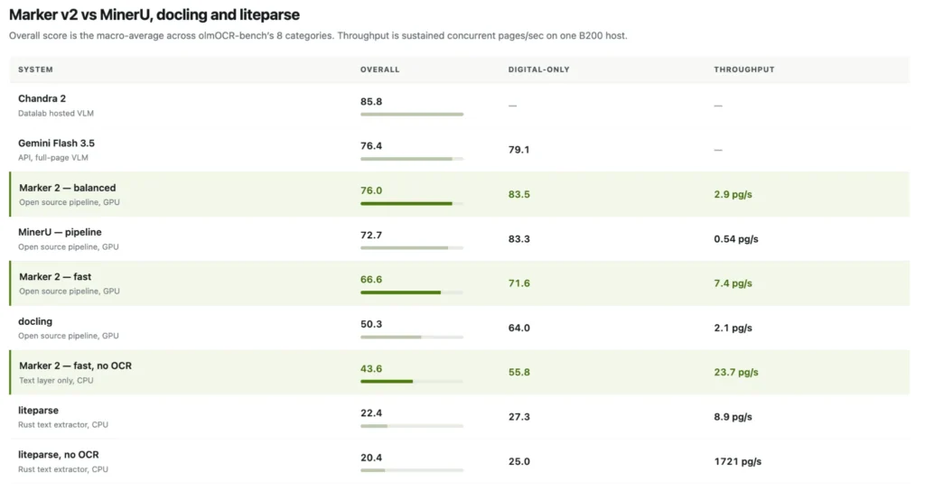
Datalab has released Marker 2, a full rewrite of its open source document conversion pipeline. Marker converts PDF, image, PPTX, DOCX, XLSX, HTML, and EPUB files into markdown, JSON, HTML, or chunks. The Datalab team rebuilt it around three components shipped over the preceding months: Surya OCR 2, a 20M-param fast layout model, and a rebuilt pdftext that is 3× faster than the previous one. The main result comes from olmOCR-bench, a third-party benchmark from Allen AI. Marker 2’s balanced mode scores 76.0% overall and 83.5% on born-digital PDFs. It sustains 2.9 pages per second on a single B200 GPU. That is over 5× the throughput of MinerU’s pipeline backend, which scores 72.7% at 0.54 pages per second. Docling scores 50.3% at 2.1 pages per second on the same harness. What’s New in Marker 2 Marker 2 exposes three conversion paths instead of one: balanced — the Surya VLM handles layout, and the whole page is re-OCR’d whenever embedded text is bad. Highest quality, best on GPU. 76.0% olmOCR-bench. fast — a lightweight rf-detr/onnx layout detector plus pdftext, with minimal, surgical VLM use. 66.6%, and far cheaper. –disable_ocr — pure text-layer extraction, no VLM calls at all. Runs entirely on CPU. 43.6%, 23.7 pg/s. Mode is now device-aware by default: balanced on GPU, fast on CPU/MPS, overridable with –mode. Full CPU support is the second structural change. fast –disable_ocr needs no GPU and no inference server, and the 20M layout model still reads columns, tables and headers on CPU. The third change is architectural, and it is the one that produces the throughput numbers. Many thin CPU workers share a single Surya inference server. The parent process budgets VLM concurrency across them, so throughput scales with server capacity rather than per-process VRAM. Datalab reports that balanced mode sustains ~2.9 pg/s against a ~0.3 pg/s single-stream rate on the same hardware. Breaking changes are worth flagging before an upgrade. Python 3.10+ is now required. Packaging moved from Poetry to uv, with hatchling as the build backend, though pip install marker-pdf is unchanged. The structured-extraction converter and extractors were removed; Datalab points users to the hosted API or a –use_llm workflow instead. Comparison The scoring benchmark is olmOCR-bench from Ai2: 1,403 PDFs with roughly 8,400 pass/fail unit tests covering math rendering, table structure, reading order, headers and footers, and old scans. The overall score is the macro-average across the 8 categories, computed with the official olmOCR-bench checker. Throughput is sustained concurrent pg/s on one B200 host, not single-stream latency. A note on provenance. olmOCR-bench is a third-party benchmark from Ai2, but every score and throughput figure below comes from Datalab’s own runs. All of them are reproducible through the open harness in the Marker repository, which ships competitor runners for MinerU, Docling and LiteParse alongside Marker’s own. These numbers also reflect one benchmark’s document mix measured on a single hardware setup, so results on your own documents may differ. Teams evaluating these systems should run the harness against their own corpus, which is the only way to know how the four rank on the documents they actually process. Marker 2 vs MinerU MinerU’s pipeline backend is the closest architectural match. Both read the PDF text layer and OCR selectively. On overall score, Marker balanced leads 76.0 to 72.7. On born-digital documents the two are effectively tied: 83.5 against 83.3. The separation is throughput. Marker balanced sustains 2.9 pg/s against MinerU’s 0.54 pg/s, a 5.4× gap at a higher score. Marker fast sustains 7.4 pg/s, roughly 13.7× MinerU’s pipeline rate, but scores 6.1 points below MinerU to do it. MinerU also ships a VLM backend, which Datalab states scores higher than its pipeline backend. That backend is a full-page-VLM approach and is not in this table. AI teams evaluating MinerU should benchmark that path separately. Marker 2 vs Docling Docling is the widest margin among the GPU pipelines. Marker balanced leads 76.0 to 50.3 overall and 83.5 to 64.0 on born-digital, while also running faster: 2.9 pg/s against 2.1 pg/s. Datalab notes Docling was run on its default pipeline, which uses the text layer for born-digital pages and OCR for image regions. Docling’s counterweight is governance and format breadth, not accuracy. The codebase is MIT-licensed, it originated at IBM Research, and it is hosted as a project in the LF AI & Data Foundation. Its input list also extends past documents into audio and email formats. Marker 2 vs LiteParse LiteParse, from the LlamaIndex team, is a Rust document parser. It does not compete on the same axis. On CPU it scores 22.4 overall and 20.4 with OCR off, against Marker’s CPU-only 43.6. But LiteParse with OCR disabled reports 1721 pg/s — roughly 73× Marker’s CPU mode, which is the tradeoff. Marker’s fast –disable_ocr runs a 20M layout model on CPU and still recovers structure, which is why it more than doubles a plain text dump’s score. LiteParse has no layout model and collapses on anything non-linear. Marker 2 vs the full-page VLM tier The Datalab team emphasizes that Marker is designed as a pipeline rather than a VLM, clarifying that these are distinct tools. In this evaluation, their hosted Chandra 2 scores 85.8, while Gemini Flash 3.5 via API scores 76.4. Datalab’s Chandra repository also positions Ai2’s olmOCR 2 at 82.4 and dots.ocr 1.5 at 83.9 within a separate table. For scans, math-heavy pages, and achieving top accuracy, the VLM tier remains superior to all listed pipelines. Marker’s balanced mode narrows the performance gap to just 0.4 points behind Gemini Flash 3.5 overall, and it even outperforms it on born-digital documents by a margin of 83.5 to 79.1—without requiring a per-page API call. Per-category behavior The mode you pick changes the failure profile, not just the score. Each row is one olmOCR-bench category, scored across all three modes. Math is the sharp edge: fast mode reads equations from the PDF text layer instead of VLM-OCRing them, so arXiv math falls from 83.9 to 23.4, and –disable_ocr scores 0.0 there by design.

Datalab Marker v2 vs MinerU, Docling, and Liteparse: Benchmark Breakdown Leggi l'articolo »

AI, Committee, Notizie, Uncategorized

Meet Open Dreamer: A JAX/Flax Reproduction of the Dreamer 4 World Model Pipeline, With the Full Training Recipe Published

A small group of AI researchers (Reactor) have released Open Dreamer, an open implementation of the Dreamer 4 world-model pipeline written in JAX and Flax NNX. What actually shipped Two repositories were released. next-state/open-dreamer holds the training pipeline: a causal video tokenizer, an action-conditioned latent dynamics model, rollout generation, and FVD scoring. reactor-team/open-dreamer holds a minimal local rollout harness that generates frames from an MP4 and a matching action file. A third artifact is the browser demo hosted on the Reactor runtime. It streams a generated Minecraft world in real time and exposes a Game ⟷ Dream toggle that hands the stream from the real game to the world model frame by frame. The stated objective was to reproduce the Dreamer 4 research. The research team deliberately avoided methods outside that research paper to keep the search space narrow. They started on CoinRun, a procedurally generated 2D platformer trainable on a single GPU, then scaled the working pipeline to Minecraft/VPT-style gameplay video. Architecture: one backbone, two models Both the tokenizer and the dynamics model use the same block-causal transformer backbone. That backbone alternates two attention types. Space layers propagate information among the elements of a single frame. Causal time layers propagate information between frames. The tokenizer is a transformer-based Masked Autoencoder rather than a VAE. The team reports roughly 100× compression and notes the design needs no KL or adversarial loss. Masking, they argue, makes the latent space more diffusible. The dynamics model performs next-frame prediction and is trained with diffusion forcing, flow matching, and shortcut models. It also predicts the next action. Rather than alternating between a separate transition module and policy, the rollout is folded into per-timestep blocks of (previous action, state, policy). Spatial attention runs inside each block; causal temporal attention connects blocks across time. Critically, world-model tokens cannot read the agent token. Task and policy information can therefore influence future states only through the next action. The training recipe, as configured The shipped Minecraft configs make the recipe concrete. The dynamics model is 1.6B parameters: 30 block-causal layers, d_model 1920, 30 attention heads, and 3 KV heads for grouped-query attention. Every fourth layer is a time-attention layer. Each timestep carries 32 learned register tokens, and packing_factor: 2 packs neighbouring tokenizer latents into each dynamics spatial token. Time attention uses a 192-step sliding window. Training runs for 200,000 steps with Muon, a WSD schedule, and a peak learning rate of 3e-4. Shortcut/bootstrap samples switch on at step 100,000 at a 0.25 batch fraction. EMA decay is 0.999. The tokenizer config emits 512 latent tokens per frame at a bottleneck width of 16. Raw 360×640 frames are padded to 368×640 so both dimensions divide into 16×16 patches. Encoder depth is 12 at d_model 1536; decoder depth is 8 at d_model 1024. MAE masking probability tops out at 0.9, and LPIPS is applied at weight 0.2 on half the timesteps. VPT actions are parsed into 27 binary action channels plus 121 categorical mouse classes, with no continuous channels. Computemaxxing and the memory wall The research team reports 57–58% model FLOPs utilization, against a stated 60% benchmark for healthy transformer training. The reasoning is a roofline argument. On a B200, the crossover between bandwidth-bound and compute-bound sits at 292 FLOP/byte. Feeding 256 frames per GPU pushes the workload past that ridge point. Sharding went the other way from expectations. At 1.6B parameters the model state — parameters, gradients, optimizer state, and EMA — occupied roughly 24 GiB, which fits on a B200. Activations were the real cost. The research team tried data parallelism, FSDP, tensor parallelism, and sequence parallelism, then settled on plain data parallelism plus activation checkpointing. Dataloading was solved by pre-tokenizing the entire dataset into .arrayrecord files, then using Grain with a GPU-side prefetch buffer. ffmpeg decoding was not fast enough to keep the GPUs fed. The stability section is the real payload The research team is explicit that stability consumed the largest share of their time. Their key observation: most stability problems occur despite the loss going down. MSE improves smoothly while generation quality degrades. Six fixes are documented. Muon replaced LaProp, which spiked randomly and increasingly often, across two runs of roughly 400 B200 hours each. EMA weights are treated as mandatory for diffusion inference. Mixed precision is boundary-sensitive: parameters stay float32, BF16 covers most matmul activations and attention inputs, and float32 is kept for normalization and the dynamics flow output head. On loss weighting, they use x-prediction with a v-space loss, which reduces to a weighting term similar to Dreamer 4’s but with a squared denominator. They report a small but noticeable improvement. Minibatch barycentric optimal transport between noise and latent sequences made rollout generation more stable. μ-parametrization was tested and judged unnecessary, partly because Muon holds hyperparameters steadier across model sizes. One further result from the CoinRun phase: an iso-FLOPs sweep put compute-optimal scaling at roughly N∝C0.56 and D∝C0.44. What is not in the box The repository does not include the behaviour-cloning or RL training loop; a full Dreamer 4 BC/RL agent loop is listed as an open roadmap item. The CoinRun policy work described in the post was not used for Minecraft and was not released. The post also does not publish FVD scores, though scripts/eval_fvd.py ships with an I3D-based harness configured for 4 context frames and a 240-frame horizon. Key Takeaways Open Dreamer reproduces the Dreamer 4 pipeline in JAX/Flax NNX, with training code and a Minecraft demo. The dynamics model is 1.6B parameters, 30 layers, d_model 1920, trained 200K steps with Muon. Reported engineering numbers: 57–58% MFU on B200, 256 frames per GPU, ~24 GiB model state. Stability, not throughput, was the bottleneck; loss curves hid most generation-quality regressions. Check out the blog post and demo, the training repo, the inference repo, and Reactor on X. All credit for this research goes to the researchers of this project. The post Meet Open Dreamer: A JAX/Flax Reproduction of the Dreamer 4 World Model Pipeline, With the Full Training Recipe Published appeared first

Meet Open Dreamer: A JAX/Flax Reproduction of the Dreamer 4 World Model Pipeline, With the Full Training Recipe Published Leggi l'articolo »

AI, Committee, Notizie, Uncategorized

Designing High-Performance GPU Kernels with TileLang: Tensor-Core GEMM, Fused Softmax, FlashAttention, and Autotuning

In this tutorial, we explore TileLang as a high-level Python domain-specific language for designing and compiling performance-oriented GPU kernels through TVM. We begin by validating the CUDA environment and establishing reusable benchmarking and numerical-verification utilities, then progressively implement vector addition, tiled tensor-core matrix multiplication, schedule exploration, fused GEMM epilogues, row-wise softmax, and FlashAttention. Throughout the tutorial, we work directly with TileLang’s shared-memory tiles, register fragments, pipelined loops, parallel iteration primitives, reductions, and tensor-core GEMM operators while allowing the compiler to manage thread mapping, memory layouts, synchronization, vectorization, and low-level CUDA instruction generation. We also compare our kernels against PyTorch and cuBLAS baselines, inspect generated CUDA source, evaluate memory and compute throughput, and use autotuning to identify architecture-dependent kernel configurations. Copy CodeCopiedUse a different Browser import os import sys import math import time import subprocess import traceback def _sh(cmd: str) -> int: print(f”$ {cmd}”, flush=True) return subprocess.run(cmd, shell=True).returncode def _bootstrap(): “””Install tilelang if missing. Stable wheel first, nightly as a fallback.””” try: import tilelang return except ImportError: pass print(“>> installing tilelang (this pulls a bundled TVM, ~1-3 min)n”) _sh(f”{sys.executable} -m pip install -q tilelang”) try: import tilelang return except ImportError: print(“>> stable wheel unusable, trying nightly channel”) _sh(f”{sys.executable} -m pip install -q tilelang ” f”-f https://tile-ai.github.io/whl/nightly”) import tilelang if os.path.isdir(“/usr/local/cuda”): os.environ.setdefault(“CUDA_HOME”, “/usr/local/cuda”) os.environ[“PATH”] = os.environ.get(“PATH”, “”) + “:/usr/local/cuda/bin” _bootstrap() import torch import torch.nn.functional as F import tilelang import tilelang.language as T def banner(title: str): print(“n” + “=” * 78) print(f” {title}”) print(“=” * 78, flush=True) def bench(fn, warmup: int = 10, rep: int = 50) -> float: “””Median-ish latency in milliseconds, measured with CUDA events.””” for _ in range(warmup): fn() torch.cuda.synchronize() start, end = torch.cuda.Event(True), torch.cuda.Event(True) start.record() for _ in range(rep): fn() end.record() torch.cuda.synchronize() return start.elapsed_time(end) / rep def check(actual: torch.Tensor, ref: torch.Tensor, name: str, tol: float = 2e-2) -> bool: “””Relative-Frobenius-norm check. Far more meaningful than atol for fp16.””” a, r = actual.float(), ref.float() rel = (a – r).norm() / r.norm().clamp_min(1e-12) amax = (a – r).abs().max().item() ok = bool(rel < tol) and math.isfinite(amax) print(f” [{‘PASS’ if ok else ‘FAIL’}] {name}: rel_err={rel:.3e} max_abs={amax:.3e}”) return ok banner(“0. ENVIRONMENT”) assert torch.cuda.is_available(), “No GPU. Runtime -> Change runtime type -> GPU.” DEV = torch.device(“cuda”) PROPS = torch.cuda.get_device_properties(0) CC = torch.cuda.get_device_capability(0) SM = CC[0] * 10 + CC[1] print(f” tilelang : {getattr(tilelang, ‘__version__’, ‘unknown’)}”) print(f” torch : {torch.__version__}”) print(f” GPU : {PROPS.name} (sm_{SM}, {PROPS.multi_processor_count} SMs, ” f”{PROPS.total_memory/2**30:.1f} GiB)”) SMEM_CAP = 48 * 1024 if SM < 80 else 96 * 1024 DEFAULT_STAGES = 2 if SM < 80 else 3 print(f” smem budget: {SMEM_CAP//1024} KB/block, default num_stages={DEFAULT_STAGES}”) print(” note: tilelang caches compiled kernels in ~/.tilelang/cache, so a”) print(” second run of this cell is dramatically faster.”) @tilelang.jit(out_idx=[-1]) def make_vector_add(N: int, block_N: int = 256, dtype: str = “float32”): @T.prim_func def main(A: T.Tensor((N,), dtype), B: T.Tensor((N,), dtype), C: T.Tensor((N,), dtype)): with T.Kernel(T.ceildiv(N, block_N), threads=256) as bx: for i in T.Parallel(block_N): C[bx * block_N + i] = A[bx * block_N + i] + B[bx * block_N + i] return main def section_1(): banner(“1. HELLO, TILE — vector add + generated CUDA”) N = 1 << 22 add = make_vector_add(N, block_N=256) a = torch.randn(N, device=DEV) b = torch.randn(N, device=DEV) c = add(a, b) check(c, a + b, “vector_add”) ms = bench(lambda: add(a, b)) gbs = 3 * N * 4 / (ms * 1e-3) / 1e9 ref_ms = bench(lambda: a + b) print(f” tilelang: {ms*1e3:8.1f} us ({gbs:6.1f} GB/s)”) print(f” torch : {ref_ms*1e3:8.1f} us <- both are pure bandwidth, so a tie” f” is the correct outcome”) src = add.get_kernel_source() print(“n — generated device code (first 32 lines) —“) for line in src.splitlines()[:32]: print(” ” + line) print(” ———————————————“) We configure the Google Colab CUDA environment, install TileLang with a nightly fallback, and import the required PyTorch and TileLang modules. We define reusable benchmarking, validation, and reporting utilities that measure kernel latency and compare numerical outputs using relative error. We then implement a TileLang vector-add kernel, execute it on the GPU, compare its bandwidth with PyTorch, and inspect the CUDA source generated by the compiler. Copy CodeCopiedUse a different Browser @tilelang.jit(out_idx=[-1]) def make_matmul(M: int, N: int, K: int, block_M: int = 128, block_N: int = 128, block_K: int = 32, num_stages: int = 3, threads: int = 128, use_swizzle: bool = False, dtype: str = “float16”, accum_dtype: str = “float”): @T.prim_func def main(A: T.Tensor((M, K), dtype), B: T.Tensor((K, N), dtype), C: T.Tensor((M, N), dtype)): with T.Kernel(T.ceildiv(N, block_N), T.ceildiv(M, block_M), threads=threads) as (bx, by): A_shared = T.alloc_shared((block_M, block_K), dtype) B_shared = T.alloc_shared((block_K, block_N), dtype) C_local = T.alloc_fragment((block_M, block_N), accum_dtype) if use_swizzle: T.use_swizzle(panel_size=10, enable=True) T.clear(C_local) for ko in T.Pipelined(T.ceildiv(K, block_K), num_stages=num_stages): T.copy(A[by * block_M, ko * block_K], A_shared) T.copy(B[ko * block_K, bx * block_N], B_shared) T.gemm(A_shared, B_shared, C_local) T.copy(C_local, C[by * block_M, bx * block_N]) return main def smem_bytes(block_M, block_N, block_K, stages, itemsize=2): return (block_M * block_K + block_K * block_N) * itemsize * stages def section_2(): banner(“2. MEMORY HIERARCHY — tiled tensor-core GEMM”) M = N = K = 2048 bm, bn, bk, st = 128, 128, 32, DEFAULT_STAGES while smem_bytes(bm, bn, bk, st) > SMEM_CAP and st > 1: st -= 1 print(f” config: {bm}x{bn}x{bk}, num_stages={st}, ” f”smem={smem_bytes(bm,bn,bk,st)/1024:.0f} KB”) kernel = make_matmul(M, N, K, bm, bn, bk, num_stages=st, threads=128) a = torch.randn(M, K, device=DEV, dtype=torch.float16) b = torch.randn(K, N, device=DEV, dtype=torch.float16) c = kernel(a, b) check(c, a @ b, “matmul 2048^3″) flops = 2 * M * N * K ms = bench(lambda: kernel(a, b)) ms_ref = bench(lambda: a @ b) print(f” tilelang : {ms:7.3f} ms -> {flops/(ms*1e-3)/1e12:6.2f} TFLOP/s”) print(f” cuBLAS : {ms_ref:7.3f} ms -> {flops/(ms_ref*1e-3)/1e12:6.2f} TFLOP/s”) print(f” ratio : {ms_ref/ms*100:5.1f}% of cuBLAS from ~20 lines of Python”) src = kernel.get_kernel_source() for needle in (“mma.sync”, “wgmma”, “ldmatrix”, “cp.async”, “tl::gemm”): if needle in src: print(f” emitted: {needle}”) return kernel def section_3(): banner(“3. KNOBS — sweeping the schedule by hand”) M = N = K = 2048 a = torch.randn(M, K, device=DEV, dtype=torch.float16) b = torch.randn(K, N, device=DEV, dtype=torch.float16) flops = 2 * M * N * K candidates = [ (64, 64, 32, 2, 128, False), (128, 128, 32,

Designing High-Performance GPU Kernels with TileLang: Tensor-Core GEMM, Fused Softmax, FlashAttention, and Autotuning Leggi l'articolo »

We use cookies to improve your experience and performance on our website. You can learn more at Politica sulla privacy and manage your privacy settings by clicking Settings.

Privacy Preferences

You can choose your cookie settings by turning on/off each type of cookie as you wish, except for essential cookies.

Allow All
Manage Consent Preferences
  • Always Active

Save
it_IT