YouZum

Committee

AI, Committee, 新闻, Uncategorized

Trajectory Releases a Concurrent Multi-LoRA Training Stack for Continual Learning, Reporting a 2.81× Experiment-Throughput Gain

Trajectory’s concurrent multi-LoRA stack reports a 2.81× experiment-throughput gain over single-tenant RL, with all code in the NovaSky-AI/SkyRL GitHub repository. Most language models improve in discontinuous jumps. A team collects data, trains, and ships a new version. This takes months and produces remarkable or catastrophic behavior for users. Trajectory wants to replace that cycle with continual learning. The Trajectory team published a field report describing how. It built a concurrent, multi-LoRA training platform for continuously learning workloads. The work was done with UC Berkeley Sky Lab and Anyscale. All training code is open-sourced in the NovaSky-AI/SkyRL repository. The result is a 2.81× end-to-end experiment-throughput improvement. The comparison is against a single-tenant training framework. Trajectory reports no regression on any training rewards. What Multi-LoRA Training Actually Is Continual learning requires models to update from live feedback and production interactions. A coding agent could learn engineering patterns as developers correct its work. A support agent could resolve hard tickets as operators intervene on difficult cases. Most training infrastructure still assumes a linear lifecycle. Teams allocate GPUs, initialize the model, run a job, then spin down. Continual learning revises that relationship. When production interactions become training inputs, training becomes part of a live system. Modern RL training reduces to three core primitives. The Sampler generates trajectories from the current policy model. The Trainer computes gradients and updates the policy weights. Parameter synchronization broadcasts updated weights back to inference workers. Trajectory calls its approach Continuous Multi-LoRA Training, or C-LoRA. Each experiment maps to a dedicated LoRA adapter on a warm, multi-tenant engine. The Problems It Targets The Trajectory team identifies four inefficiencies in traditional stacks: (1) Cold starts are slow: Every serial job reloads checkpoints, initializes the distributed runtime, and warms inference engines. For large models, this step alone can exceed 30 minutes per run. (2) RL is memory intensive: Frontier models often exceed 100B parameters. Qwen3.5-397B can require up to eight H200 nodes to fit into memory. LoRA cuts memory usage by an order of magnitude. It freezes the base model and trains only small adapter weights. (3) Traditional stacks are single-tenant: They run one experiment at a time. Multi-LoRA maps each experiment to one adapter, multiplexing throughput by a factor of N. (4) Job utilization is low: Trainers and inference engines stall while waiting for each other. Multi-LoRA load balances across jobs to fill idle capacity. Inside the Architecture Most throughput wins come from inference. In vLLM, all adapters are hot-loaded in GPU memory. Decode steps can then mix tokens from different adapters in the same batch. The key enabler is the SGMV decode kernel. It fuses per-adapter matrix-vector work into one GPU launch per decode step. After each optimization step, updated LoRA weights load in-place into the inference engine. The scheduler does not freeze, so other tenants keep decoding. Training works differently. One active LoRA adapter trains on the GPU. The rest sit in pinned CPU memory. Each tenant’s state lives in an AdapterStore. It holds LoRA parameters, FP32 master weights, optimizer moments, and gradient buffers. The engine swaps one tenant’s state onto the GPU, runs a single forward_backward pass, then swaps it back. This training path is still single-adapter. The inference concurrency gains do not yet apply to training. The Numbers Trajectory tested on a single H200 node with Qwen3-4B-Instruct-2507. It ran sync RL on GSM8K in an agentic setting. The Trajectory team reframed GSM8K as a tool use learning task. The model decides when to call a Calculator and a Final Answer tool. Reward is 1.0 only when Final Answer is called with the correct answer. The policy starts near 40% accuracy at step 0. With the right learning algorithm, it climbs past 90% by step 9. The Trajectory team scaled to eight concurrent multi-LoRA runs. Final Experiment Time hit 5433s at N=8, a 2.81× speedup. Eight concurrent experiments finished before three serial runs back-to-back. Mean Experiment Time also improved, peaking at N=4 with a 1.88× speedup. Every concurrency level reached reward_accuracy above 90% by step 9. The Tradeoffs Higher throughput costs per-step latency. As N grows, First Experiment Time and Step Time degrade. At N=8, the first serial experiment finishes 1.97× faster. Mean step time rises from 191s to 500s, only 2.62× slower. Most of that increase is rollout time. Rollout grows from 162s to 401s, roughly 77% of the increase. At N=2, doubling the load adds only 15% rollout time. That is the ideal case for multi-LoRA. The pattern held on a harder workload. On τ-bench retail with the NVIDIA-Nemotron-3-Nano-30B-A3B-BF16 MoE model, N=2 finished 10 steps 1.28× faster. Per-tenant step time rose 1.57×. Strengths and Weaknesses Strengths: 2.81× end-to-end experiment-throughput gain at eight concurrent runs No accuracy regression; runs tracked the serial baseline within ±1σ in the final steps LoRA cuts memory by an order of magnitude versus full fine-tuning Fully open-sourced in NovaSky-AI/SkyRL for the community to build on Weaknesses: Per-step latency and First Experiment Time degrade as N grows Training remains serialized across tenants; only inference is multiplexed Tested mainly on mid-sized models, not frontier-scale parameters Setup requires an 8× H100/H200 node and a Megatron build Key Takeaways Trajectory built a concurrent, multi-LoRA RL training stack for continual learning, open-sourced in NovaSky-AI/SkyRL. It reports a 2.81× end-to-end experiment-throughput gain over a single-tenant baseline, with no reward regression. Each experiment maps to a dedicated LoRA adapter on an always-hot engine, multiplexing throughput by N. Most gains come from vLLM multi-LoRA inference via the SGMV decode kernel; training stays single-adapter. The tradeoff is per-step latency: at N=8, step time rises from 191s to 500s. Marktechpost’s Visual Explainer Field Report · May 27, 2026 Continuous Multi-LoRA Training for Continual Learning Trajectory, built with UC Berkeley Sky Lab and Anyscale. 2.81× end-to-end experiment-throughput gain Training code open-sourced in the NovaSky-AI/SkyRL repository. 01 — What it is One always-hot engine, many adapters Continual learning updates models from live feedback and production interactions. Trajectory calls its approach Continuous Multi-LoRA Training (C-LoRA). Each experiment maps to a dedicated LoRA adapter on
Trajectory Releases a Concurrent Multi-LoRA Training Stack for Continual Learning, Reporting a 2.81× Experiment-Throughput Gain Read Post »

AI, Committee, 新闻, Uncategorized

Best Text-to-Speech TTS Models in 2026: A Benchmark-Based Comparison

Text-to-speech TTS moved fast over the past year. The line between synthetic and human speech narrowed. Latency dropped below 100 milliseconds for some real-time systems. Emotional control became a standard feature rather than a research demo. This guide reviews the models that really matter in 2026. It is written for AI professionals choosing a model for production. How to read TTS benchmarks in 2026 Two benchmarks dominate in most community discussions. The first is the Artificial Analysis Speech Arena Leaderboard. It ranks models by blind human preference using an ELO rating. As of 2026 it evaluates dozens of production APIs. The second is the community-run TTS Arena on Hugging Face. It uses the same blind A/B voting method. These leaderboards measure perceived quality, not accuracy. They also change continuously. As of May 30, 2026, the Artificial Analysis Speech Arena lists Gemini 3.1 Flash TTS, Realtime TTS-2 (Research Preview), Sonic 3.5, Realtime TTS 1.5 Max, and Fun-Realtime-TTS-Preview as its top five by ELO. Those positions shifted within the prior weeks, and they will shift again. Treat any single number as a point-in-time reading, not a fixed truth. Accuracy needs separate measurement. Trelis Research tested ten models using a round-trip character error rate, or CER. The method transcribes generated audio with an ASR model, then compares it to the input text. Mean opinion score, or MOS, captures perceived naturalness. Both metrics have limits. Round-trip CER depends on the ASR model’s own accuracy. The UTMOS quality estimator was trained on audio up to ten seconds, so longer samples show less score spread. Latency is the third axis. The relevant figure for voice agents is time-to-first-audio, or TTFA. Time-to-first-byte, or TTFB, can be misleading, since container headers carry no audio. Consistency matters as much as the median. A Gradium benchmark from May 2026 measured the interquartile range across providers. Tail latency, not the average, determines user experience at scale. In short, no benchmark is complete. Quality, accuracy, latency, language coverage, and price all trade off. The right model depends on which axis your application cannot compromise. Commercial leaders #1 Inworld TTS-1.5 and Realtime TTS-2 Inworld AI is a research lab founded by a team from Google and DeepMind. It released TTS-1.5 on January 21, 2026. The model targets real-time, consumer-scale applications. Inworld reports roughly 30 percent more expressive range than TTS-1. It also reports about 40 percent better stability, measured through word error rate and output consistency. TTS-1.5 ships in two tiers. The Mini tier is tuned for latency-sensitive workloads such as voice agents and gaming. The Max tier balances higher stability with low latency. Inworld reports P90 time-to-first-audio under 130 milliseconds for Mini and under 250 milliseconds for Max. The model supports 15 languages and offers both instant and professional voice cloning. Pricing is tiered by plan, not a single rate. On the On-Demand and Creator plans, Inworld lists $25 per million characters for TTS 1.5 Mini and $35 for Realtime TTS-2 and TTS 1.5 Max. The Developer and Growth plans cut those rates; Growth reaches $15 for Mini and $25 for Max and TTS-2. Enterprise pricing goes as low as $5 and $10 respectively. Note that TTS 1.5 covers 15 languages, while TTS-2 covers over 100. Inworld later added Realtime TTS-2 in 2026. It is described as a closed-loop voice model with stronger steering and expressiveness. Across several leaderboard snapshots, Inworld reported holding three of the top five spots on the Artificial Analysis Speech Arena. Inworld suits developers building voice agents at consumer scale. The combination of low latency and aggressive pricing is its main draw. #2 Google Gemini 3.1 Flash TTS Google DeepMind released Gemini 3.1 Flash TTS on April 15, 2026. It is a preview model available through the Gemini API, Google AI Studio, Vertex AI, and Google Vids. The model introduces more than 200 audio tags. These tags steer style, tone, pacing, accent, and scene direction. On Google’s own report, the model reached an ELO of 1,211 on the Artificial Analysis leaderboard. It supports 70-plus languages and native multi-speaker dialogue. Google built it on the Gemini family rather than a standalone speech stack. The model treats generation as a language task: it decides not only what to say, but how to say it. The model has documented limitations that matter for deployment. A TTS session has a 32,000-token context window, and Google’s docs state that Gemini TTS does not support streaming. It is built for controlled text recitation, not interactive voice agents; the separate Live API is Google’s real-time path. Output quality can drift on generations longer than a few minutes, so Google recommends chunking. The model offers 30 prebuilt voices. All generated audio carries a SynthID watermark for AI-content identification. Gemini 3.1 Flash TTS fits podcast and audiobook generation with fine-grained control. It is a strong default for teams already on Google Cloud. #3 ElevenLabs v3 ElevenLabs released Eleven v3 in alpha on June 5, 2025. It reached general availability in early 2026, per the company’s announcement. ElevenLabs describes it as its most expressive model. It introduced inline audio tags formatted in lowercase square brackets. Examples include [whispers], [laughs], [sighs], and scene cues like [interrupting]. The model supports more than 70 languages. The GA release refined the alpha. ElevenLabs reports users preferred the new version about 72 percent of the time. It also improved how the model handles numbers, symbols, and specialized notation. A key feature is Text to Dialogue. It weaves multiple voices into one generation pass. The model matches prosody and emotional range across speakers. It can handle interruptions and shifting moods with limited prompting. Eleven v3 still requires more prompt engineering than earlier models. It is not built for real-time use. ElevenLabs states the larger model and higher-fidelity codec take longer to run. For real-time and conversational use, the company recommends Flash v2.5 instead. Those models stream with low latency, around the 75-millisecond range in vendor figures. ElevenLabs v3 fits narrative content, audiobooks, and character work where quality outweighs speed. It remains a common

Best Text-to-Speech TTS Models in 2026: A Benchmark-Based Comparison Read Post »

AI, Committee, 新闻, Uncategorized

A Coding Implementation on Loguru for Designing Robust, Structured, Concurrent, and Production-Ready Python Logging Pipelines

In this tutorial, we implement a practical use case with Loguru, a powerful, flexible, and production-ready logging library for Python. We start by building a clean, idempotent logging setup that can be safely rerun without duplicating handlers or producing messy output. From there, we move step by step through structured logging, contextual logging, custom log levels, global patching, callable formatters, and in-memory sinks. We also handle real-world logging needs such as rich exception traces, JSON log files, custom rotation, compression, retention, async logging, threaded execution, multiprocessing-safe logging, and standard logging module interception. By keeping everything in a Colab-ready workflow, we make it easy to test, inspect, and understand how Loguru can support debugging, monitoring, and observability in serious Python applications. Copy CodeCopiedUse a different Browser !pip install -q loguru nest_asyncio import os, sys, time, json, glob, gzip, shutil, asyncio, logging, itertools, multiprocessing from collections import deque from concurrent.futures import ThreadPoolExecutor, ProcessPoolExecutor from loguru import logger try: import nest_asyncio; nest_asyncio.apply() except Exception as e: print(“nest_asyncio not applied:”, e) WORKDIR = “/content/loguru_demo” if os.path.isdir(“/content”) else “/tmp/loguru_demo” os.makedirs(WORKDIR, exist_ok=True); os.chdir(WORKDIR) for f in glob.glob(“*”): try: os.remove(f) except OSError: pass print(f”Working directory: {WORKDIR}n”) RESULTS = [] def check(name, condition, detail=””): ok = bool(condition); RESULTS.append((name, ok)) print(f” [{‘PASS’ if ok else ‘FAIL’}] {name}” + (f” — {detail}” if detail else “”)) def banner(t): print(f”n{‘=’*64}n {t}n{‘=’*64}”) _seq = itertools.count(1) def global_patcher(record): record[“extra”].setdefault(“env”, “colab”) record[“extra”][“seq”] = next(_seq) _NOISE = {“env”, “seq”, “app”} def console_formatter(record): fmt = (“<green>{time:HH:mm:ss.SSS}</green> | <level>{level: <8}</level> | ” “<cyan>{name}:{function}:{line}</cyan> – <level>{message}</level>”) if any(k not in _NOISE for k in record[“extra”]): fmt += ” | <yellow>{extra}</yellow>” return fmt + “n{exception}” We install Loguru and supporting dependencies, import all required libraries, and prepare a clean working directory for the tutorial. We also create a small verification helper to test each feature as the tutorial runs. We then define a global patcher and console formatter so that every log record carries useful metadata and appears in a readable format. Copy CodeCopiedUse a different Browser class MemorySink: def __init__(self, capacity=2000): self.buffer = deque(maxlen=capacity) def write(self, message): self.buffer.append(message.record) def flush(self): pass def has_level(self, name): return any(r[“level”].name == name for r in self.buffer) def find(self, pred): return [r for r in self.buffer if pred(r)] MAX_BYTES = 1500 def size_rotation(message, file): return file.tell() + len(message) > MAX_BYTES def gzip_compression(filepath): with open(filepath, “rb”) as fi, gzip.open(filepath + “.gz”, “wb”) as fo: shutil.copyfileobj(fi, fo) os.remove(filepath) def keep_latest_retention(files): for old in sorted(files, key=os.path.getmtime, reverse=True)[3:]: try: os.remove(old) except OSError: pass class InterceptHandler(logging.Handler): def emit(self, record): try: level = logger.level(record.levelname).name except ValueError: level = record.levelno frame, depth = logging.currentframe(), 2 while frame and frame.f_code.co_filename == logging.__file__: frame, depth = frame.f_back, depth + 1 (logger.opt(depth=depth, exception=record.exc_info) .bind(stdlib_logger=record.name) .log(level, record.getMessage())) def mp_worker(n): logger.bind(child=os.getpid()).info(“hello from child item {}”, n) return os.getpid() We create reusable logging components that make the tutorial more practical and production-like. We define an in-memory sink, custom file rotation, compression, and retention functions to control how logs are stored. We also built a standard logging interceptor and a multiprocessing worker to connect Loguru to external libraries and child processes. Copy CodeCopiedUse a different Browser banner(“1) logger.configure(): handlers + custom level + extra + patcher”) mem = MemorySink() logger.configure( handlers=[ {“sink”: sys.stderr, “format”: console_formatter, “level”: “DEBUG”, “colorize”: True, “backtrace”: True, “diagnose”: True}, {“sink”: mem, “level”: “DEBUG”, “format”: “{message}”}, {“sink”: “structured.jsonl”, “serialize”: True, “level”: “DEBUG”, “enqueue”: True}, {“sink”: “errors.log”, “level”: “ERROR”, “enqueue”: True, “backtrace”: True, “diagnose”: False, “format”: “{time:YYYY-MM-DD HH:mm:ss} | {level} | ” “{name}:{function}:{line} | {message}”}, ], levels=[{“name”: “NOTICE”, “no”: 22, “color”: “<blue><bold>”, “icon”: “”}], extra={“app”: “loguru-advanced”}, patcher=global_patcher, ) logger.debug(“debug”); logger.info(“info”); logger.success(“SUCCESS level ships built-in”) logger.warning(“warning”); logger.log(“NOTICE”, “custom level between INFO and SUCCESS”) banner(“2) bind() / contextualize() / patch()”) logger.bind(user_id=42, request_id=”abc-123″).info(“bound context”) with logger.contextualize(task=”batch-job”, run=7): logger.info(“inside contextualized block”) logger.patch(lambda r: r[“extra”].update(epoch=round(time.time()))).info(“per-call patched record”) banner(“3) @logger.catch + context-manager form”) def inner(d): return d[“a”] / d[“b”] def outer(d): return inner(d) @logger.catch(reraise=False) def compute(d): return outer(d) compute({“a”: 1, “b”: 0}) with logger.catch(message=”handled inside a with-block”): raise ValueError(“boom in block”) banner(“4) opt(lazy=True), inline colors, record access”) logger.opt(lazy=True).debug(“lazy sum = {}”, lambda: sum(i*i for i in range(1_000_000))) logger.opt(colors=True).info(“inline <red>colors</red> <green>work</green>”) logger.opt(record=True).info(“emitted from source line {record[line]}”) We configure Loguru with multiple handlers, including console output, memory capture, JSON logging, and error logging. We then demonstrate structured logging with bound context, contextual blocks, patched records, and a custom log level. We also explore exception handling and useful opt() features such as lazy evaluation, inline colors, and record access. Copy CodeCopiedUse a different Browser banner(“5) custom rotation/compression/retention (forces real rotation)”) ev_id = logger.add(“events_{time:HHmmss_SSS}.log”, rotation=size_rotation, compression=gzip_compression, retention=keep_latest_retention, enqueue=True, level=”DEBUG”, format=”{time:HH:mm:ss.SSS} | {level: <8} | {message}”) for i in range(80): logger.bind(idx=i).debug(“rotating event line number {}”, i) logger.complete(); logger.remove(ev_id) print(f” archives created: {sorted(glob.glob(‘events_*.gz’))}”) banner(“6a) ThreadPoolExecutor with per-thread contextualize()”) thread_caps = [] tid = logger.add(thread_caps.append, level=”DEBUG”, format=”{message}”, filter=lambda r: “worker_id” in r[“extra”]) def worker(n): with logger.contextualize(worker_id=n): logger.info(“thread work item {}”, n) return n * n with ThreadPoolExecutor(max_workers=8) as ex: sq = list(ex.map(worker, range(8))) logger.complete(); logger.remove(tid) worker_ids = {m.record[“extra”][“worker_id”] for m in thread_caps} banner(“6b) async coroutine sink + await logger.complete()”) async def run_async_demo(): sunk = [] async def async_sink(message): await asyncio.sleep(0); sunk.append(message.record[“message”]) sid = logger.add(async_sink, level=”DEBUG”, catch=True) async def task(n): with logger.contextualize(coro=n): logger.info(“async task {} start”, n) await asyncio.sleep(0.01) logger.success(“async task {} done”, n) await asyncio.gather(*(task(i) for i in range(5))) await logger.complete() logger.remove(sid) return sunk try: async_msgs = asyncio.run(run_async_demo()) except RuntimeError: async_msgs = asyncio.get_event_loop().run_until_complete(run_async_demo()) print(f” async sink received {len(async_msgs)} messages”) We demonstrate custom file management by automatically rotating, compressing, and retaining log files. We then test thread-safe logging by running multiple workers, each with its own contextual metadata. We also add an asynchronous coroutine sink to see how Loguru handles async tasks and correctly drains pending logs. Copy CodeCopiedUse a different Browser banner(“7) intercept stdlib `logging` and filter a chatty library”) logging.basicConfig(handlers=[InterceptHandler()], level=0, force=True) lib_caps = [] def lib_filter(record): if record[“extra”].get(“stdlib_logger”) == “chatty”: return record[“level”].no >= logger.level(“WARNING”).no return True lid = logger.add(lib_caps.append, level=”DEBUG”, format=”{message}”, filter=lambda r: (“stdlib_logger” in r[“extra”]) and lib_filter(r)) logging.getLogger(“chatty”).info(“noisy info (should be filtered out)”) logging.getLogger(“chatty”).warning(“noisy warning (kept)”) logging.getLogger(“important”).debug(“important debug (kept)”) logger.complete(); logger.remove(lid) banner(“8) SELF-TESTS”) logger.complete(); time.sleep(0.2) try: rec = json.loads(open(“structured.jsonl”).read().splitlines()[-1]) check(“JSON sink serializes records”, {“text”,

A Coding Implementation on Loguru for Designing Robust, Structured, Concurrent, and Production-Ready Python Logging Pipelines Read Post »

AI, Committee, 新闻, Uncategorized

StepFun Releases Step 3.7 Flash: A 198B MoE Vision-Language Model for Coding Agents and Search Workflows

StepFun today released Step 3.7 Flash, a multimodal Mixture-of-Experts model targeting agentic use cases. It adds native vision input and improved tool-use reliability over Step 3.5 Flash. What is Step 3.7 Flash? Step 3.7 Flash is a 198B-parameter sparse Mixture-of-Experts (MoE) vision-language model. It pairs a 196B-parameter language backbone with a 1.8B-parameter vision encoder (ViT) for native image understanding. The model activates approximately 11B parameters per token during inference. In MoE architectures, only a subset of “expert” sub-networks fires per forward pass — not the full network. This keeps inference compute closer to an 11B dense model while maintaining a 198B total parameter budget. Key specs: Spec Value Total parameters 198B (196B language + 1.8B ViT) Active parameters per token ~11B Context window 256k tokens Throughput Up to 400 tokens/sec Reasoning levels Low, medium, high License Apache 2.0 Architecture Notes The vision encoder runs as a separate 1.8B ViT module. It injects image representations into the language backbone’s context. Step 3.5 Flash had no multimodal support; this is a new addition in 3.7. Three selectable reasoning depths — low, medium, and high — let developers trade latency for reasoning depth. Low is faster and cheaper; high applies more computation per response. Agentic Coding Performance On SWE-Bench Pro, Step 3.7 Flash scores 56.26%, up from Step 3.5 Flash’s 51.3% — a gain of roughly 5 percentage points. On Terminal-Bench 2.1, it scores 59.55%, up from 53.37%. On SWE-MTLG (a multi-task long-generation coding benchmark), it scores 72.42%. Cross-harness consistency on StepFun’s internal Step-SWE-Bench: Scaffold Step 3.7 Flash Step 3.5 Flash Hermes Agent 67.5% 60.0% OpenClaw 67.0% 47.0% KiloCode 67.5% 59.0% RooCode 64.5% 43.0% Claude Code 71.5% 73.0% OpenCode 64.5% 57.0% Step 3.5 Flash ranged from 43% to 73% across harnesses. Step 3.7 Flash ranges from 64.5% to 71.5%. In production, coding agents often run inside heterogeneous scaffolds — each with its own prompting conventions and tool schemas. Narrower per-harness variance means more predictable behavior across different setups. Advisor Mode Step 3.7 Flash supports Advisor Mode, StepFun’s implementation of the advisor strategy described by Anthropic. The model runs the agentic loop end-to-end — calling tools, reading results, iterating — and escalates to a larger advisor model only at specific inflection points, such as planning or recovering from repeated failures. Most of the run stays at executor cost. With Advisor Mode enabled on SWE-Bench Verified, StepFun reports Step 3.7 Flash reaches 97% of Claude Opus 4.6’s coding performance at roughly one-ninth the per-task cost ($0.19 vs. $1.76 per task). These are StepFun’s internal figures. Multimodal Capabilities Step 3.7 Flash supports two visual tool pathways: Visual Search Tool — For recognition tasks where the model’s parametric knowledge is insufficient (long-tail entities, recently emerged concepts), it invokes a visual search tool to retrieve and verify. On SimpleVQA (with Search), it scores 79.16%, comparable to GPT 5.5 (79.11%) and above Kimi K2.6 (78.24%) and GLM 5V Turbo (78.20%). Python Tool — For fine-grained visual tasks (high-resolution images, visual probing, bounding-box analysis), it uses a code interface to crop, zoom, and draw pixels or bounding boxes. On V (a self-tested score with Python), it scores 95.29%. On HR-Bench 4K and HR-Bench 8K, it scores 89.13% and 86.34% respectively. StepFun notes an observed behavior during testing: the model combined visual tools with non-visual tools without being explicitly trained to do so. For example, after generating frontend code, it used the GUI to render and inspect the result before iterating. StepFun describes this as emergent compositional tool use. On Android Daily (long-horizon phone UI task completion), Step 3.7 Flash scores 61.87%, ahead of Kimi K2.6 (53.36%) and GLM 5V Turbo (51.68%). Gemini 3 Flash (63.21%) leads this benchmark. Search and Research Benchmarks StepFun focused this model’s search design on planning, evidence filtering, and synthesis — integrating search as part of the reasoning loop rather than a separate add-on. Benchmark Step 3.7 Flash Notable comparison HLE with Tools (acc) 47.20% DeepSeek V4 Flash: 45.10% BrowseComp (acc) 75.82% Claude Opus 4.7: 79.30% DeepSearchQA (F1) 92.82% Kimi K2.6: 92.50% ResearchRubrics (score) 71.68% GPT 5.5: 61.50% Note: The HLE with Tools score of 47.20% compares to Step 3.5 Flash’s text-only score of 35.68%. Step 3.5 Flash did not support tool-augmented evaluation on HLE. General Agent Benchmarks Benchmark Step 3.7 Flash Description Toolathlon 49.51% Multi-tool coordination ClawEval-1.1 67.07% Daily autonomous task execution in realistic environments GDPval (44 occupations) 45.8% General professional task execution Tau2-bench Telecom >98% Across different reasoning difficulty tiers On ClawEval-1.1, Step 3.7 Flash (67.07%) leads DeepSeek V4 Flash (57.80%) and DeepSeek V4 Pro (59.80%) among the compared models. Long-Context Performance On AA-LCR (a long-context retrieval benchmark, avg@16/acc), Step 3.7 Flash scores 63.94%. This is comparable to DeepSeek V4 Flash (63.70%) and DeepSeek V4 Pro (66.30%). Pricing Token Type Price Input (cache miss) $0.20 / M tokens Input (cache hit) $0.04 / M tokens Output $1.15 / M tokens Marktechpost’s Visual Explainer Model Release Step 3.7 Flash — A 198B MoE Vision-Language Model StepFun · Released May 29, 2026 · Apache 2.0 Slide 1 of 8 — Overview What Is Step 3.7 Flash? Step 3.7 Flash is a sparse Mixture-of-Experts (MoE) vision-language model from StepFun. It combines a 196B-parameter language backbone with a 1.8B-parameter Vision Transformer (ViT) encoder for native image understanding. In a MoE model, only a subset of “expert” sub-networks activates per token — not the full network. This keeps inference compute close to an 11B dense model while maintaining 198B total parameters. Total Params 198B Active / Token ~11B Context Window 256k tokens Throughput 400 tok/sec Reasoning Levels Low / Med / High License Apache 2.0 Slide 2 of 8 — Architecture Architecture Notes The 1.8B ViT encoder runs as a separate module and injects image representations into the language backbone’s context. Step 3.5 Flash was text-only; native multimodal support is new in 3.7. Three selectable reasoning depths let developers balance speed and cost: Low — Fastest, cheapest. Suitable for simple completions. Medium — Balanced cost and reasoning depth. High — More compute per response. Best for complex agent

StepFun Releases Step 3.7 Flash: A 198B MoE Vision-Language Model for Coding Agents and Search Workflows Read Post »

AI, Committee, 新闻, Uncategorized

NVIDIA Introduces X-Token: Projection-Guided Cross-Tokenizer KD That Outperforms GOLD by +3.82 Average Points on Llama-3.2-1B

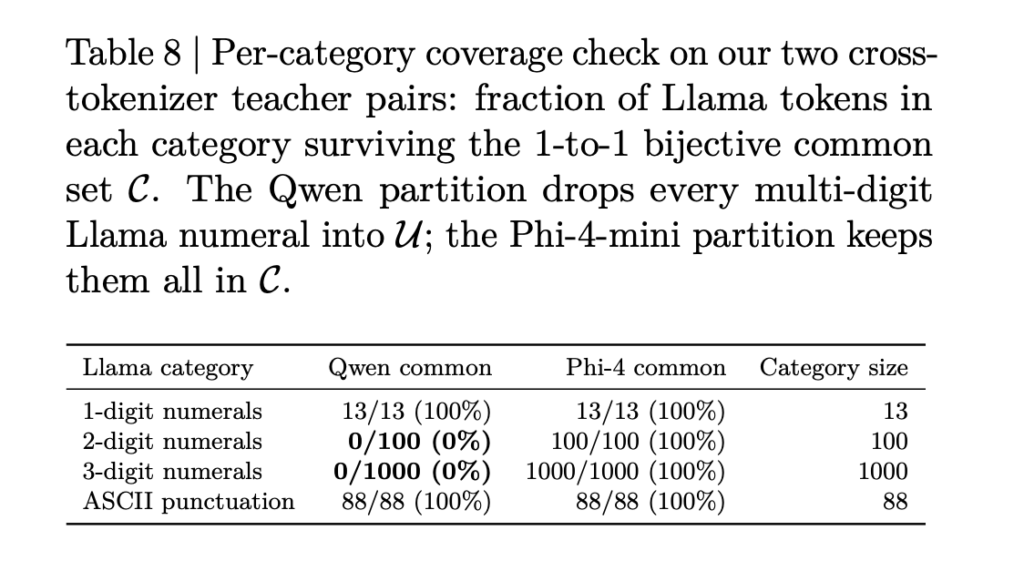
Knowledge distillation (KD) transfers “dark knowledge” from a large teacher model to a smaller student. The student learns from the teacher’s full output probability distribution over tokens, not just correct answers. This is done via per-position Kullback–Leibler (KL) divergence over next-token probability distributions. This formulation requires a shared tokenizer. A practitioner committed to Llama-3.2-1B cannot leverage stronger teachers with incompatible tokenizers — such as Phi-4-mini or Qwen3-4B — because token positions do not correspond across vocabularies. This also prevents multi-teacher distillation across tokenizer families. NVIDIA researchers introduced X-Token, a logit-distribution-based method for cross-tokenizer KD (Knowledge distillation). It operates as a drop-in replacement for the standard KD loss, requiring no auxiliary trainable components and no architectural changes. The Problem X-Token is Solving Two prior approaches dominate cross-tokenizer KD. ULD (Universal Logit Distillation) sidesteps vocabulary alignment by rank-sorting both distributions and minimizing L1 distance. It discards token identity entirely. GOLD adds span alignment and a hybrid loss. It partitions tokens into a 1-to-1 string-matched common subset, trained with KL divergence, and an uncommon remainder, trained with ULD-style rank matching. GOLD is the current state of the art. The research team identifies two structural failures in GOLD’s design: Failure 1: Uncommon-token failure– When tokenizers fragment text differently, critical tokens fall into the unmatched uncommon subset. Llama-3 packs multi-digit numbers as single tokens — “201” is one token. Qwen3 splits them digit by digit: “2”, “0”, “1”. Under GOLD, all 1,100 of Llama’s two- and three-digit numerals (100 two-digit, 1,000 three-digit) fall into the uncommon set when Qwen3-4B is the teacher. Those tokens receive two types of harmful signal: identity-agnostic noise from rank-based ULD matching, and suppressive gradients from the common-KL term acting through the full-vocabulary softmax. The result: GSM8k accuracy drops to 2.56 under GOLD with Qwen3-4B, compared to 12.89 for same-tokenizer KD from a weaker Llama-3.2-3B teacher. Failure 2: Over-conservative matching– GOLD uses strict string equality to define the common subset. A student token Hundreds corresponds to teacher tokens Hund followed by reds under teacher-side re-tokenization, but strict matching discards this pair. Useful alignment signal is lost even when the correspondence is well-formed. These two failures require opposite remedies: eliminate the partition when critical tokens are misaligned, and relax it when alignment is structurally sound. How X-Token Works X-Token has three components: span alignment, a projection matrix W, and two complementary loss formulations — P-KL and H-KL. Span Alignment Teacher and student tokenizers produce sequences of different lengths for the same text. X-Token uses dynamic-programming (DP) span alignment, grouping tokens into chunks where each chunk-pair decodes to the same underlying text substring. A chain-rule merge then combines per-token probabilities within each chunk into a single chunk-level distribution for use in the distillation loss. The alignment is cached per sequence and adds no per-step training overhead. The research team also identifies a failure in TRL’s surface-substring alignment, which is used in TRL’s GOLD trainer. TRL accumulates per-side decoded buffers and flushes only when both buffers match as equal raw strings. A byte-level disagreement — such as Llama-3 auto-prepending <bos> while Qwen-3 does not — prevents future flushes and forces all remaining tokens into one mis-grouped super-group at end of sequence. The DP approach handles this with a single gap move, regardless of sequence length. The Projection Matrix W After alignment, teacher and student distributions still operate over different vocabularies. The projection matrix W ∈ ℝVS|×|VT| maps each student token to a weighted combination of teacher tokens, bridging the vocabulary mismatch. W is constructed deterministically in two passes: Pass 1 (exact-match): For every (student token, teacher token) pair whose decoded strings match after canonicalization, set W[s, t] = 1. Canonicalization unifies space prefixes (Ġ, _, ␣), newlines, byte-fallback tokens of the form <0xHH>, and model-specific special tokens across tokenizer families. Pass 2 (multi-token rule): For each student token without an exact match, re-tokenize its decoded text under the teacher tokenizer. If the resulting sequence has length ≤ 4, assign exponentially-decayed weights: W[s, τᵢ] = β·γⁱ with (β, γ) = (0.9, 0.1). A length-2 span receives normalized weights (0.909, 0.091). A length-3 span receives (0.9009, 0.0901, 0.0090). A length-4 span receives (0.9000, 0.0900, 0.0090, 0.0009). The leading sub-token receives the highest weight because it typically carries the most informative probability mass — for example, “_inter” in [“_inter”, “national”] or “_20” in [“_20”, “24”]. Each row is truncated to its top-4 entries and row-normalized. Because each row of W is non-negative and sums to 1, left-multiplication by W⊤ is probability-preserving: if pS is a probability vector, W⊤pS is also a valid probability vector over VT. W is constructed once before training and can optionally be jointly refined with the student under P-KL. P-KL: Addressing Erroneous and Suppressive Gradients P-KL removes the partition entirely. It projects the student distribution p̂S(k) into teacher vocabulary space via W: p~S(k)[t]=∑s∈𝒱SW[s,t]⋅p^S(k)[s]tilde{p}_S^{(k)}[t] = sum_{sinmathcal{V}_S} W[s, t] cdot hat{p}_S^{(k)}[s] Then it computes KL divergence directly between teacher and projected student: ∂ℒcommon∂zj=pS[j]⋅M𝒞(T)frac{partialmathcal{L}_{common}}{partial z_{j}} = p_S[j] cdot M_{mathcal{C}}(T) There is no uncommon set, so rank-based ULD noise is eliminated. The suppressive gradient problem is also eliminated: the projection routes the student’s probability mass for “201” directly onto {2, 0, 1} in the teacher vocabulary via W. The research team formally proves (Proposition 1) that GOLD’s common-KL term induces non-negative gradients on every uncommon student logit. The gradient on an uncommon student logit j is: ∂ℒcommon/∂zj = pS[j] · MC(T), where MC(T), is the teacher probability mass on the common subset. Under gradient descent, this always drives zj downward — suppressing every uncommon token’s probability regardless of the ground-truth token. H-KL: Relaxing the 1-to-1 Matching H-KL applies when the partition is structurally sound — that is, when critical tokens land in the common subset. In that case, GOLD’s direct KL on identity-aligned pairs delivers sharper per-pair supervision than P-KL’s projection, which blends student probability mass across multiple teacher tokens. The opportunity is to make the partition less wasteful by relaxing the strict string-equality criterion. H-KL retains GOLD’s hybrid loss structure but expands the common set

NVIDIA Introduces X-Token: Projection-Guided Cross-Tokenizer KD That Outperforms GOLD by +3.82 Average Points on Llama-3.2-1B Read Post »

AI, Committee, 新闻, Uncategorized

Hermes Agent Ships Tool Search for MCP: Anthropic Evals Show 49% to 74% Accuracy Gain on Opus 4

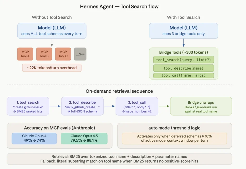
Nous Research’s open-source Hermes Agent now ships a Tool Search feature. It directly addresses a growing bottleneck in AI agent systems: too many MCP tools filling up the context window. In this explainer article, we will breaks down what Tool Search does, how it works, and when to use it. The Problem: MCP Tools Are Eating Your Context Window When you connect multiple MCP (Model Context Protocol) servers to an AI agent, every tool’s JSON schema gets sent to the model on every turn. This happens even if the model only needs one or two tools for a given task. Real-world deployments feel this immediately. A Hermes deployment with five MCP servers and 34 tools shows average prompt sizes of 45,000 tokens per turn. Roughly 22,000 of those tokens — around 50% — are tool schema overhead alone. Anthropic’s own engineering data shows tool definitions can consume 134,000 tokens before optimization. Tool Attention measures the “MCP Tools Tax” at 15,000–60,000 tokens per turn for typical multi-server deployments. This creates two distinct problems: Cost: Cache-miss generations at session start can cost $0.07–$0.10 per turn. Accuracy loss: Decision paralysis sets in when the model sees hundreds of irrelevant tool options simultaneously. Source: hermes-agent.nousresearch.com/docs · Nous Research 2026 What is Tool Search? Tool Search is Hermes Agent’s opt-in progressive-disclosure layer for MCP and non-core plugin tools. Instead of loading every tool schema upfront, the model loads only what it needs — on demand, per turn. When Tool Search activates, MCP and plugin tools are replaced in the model-visible tools array by three bridge tools: Copy CodeCopiedUse a different Browser tool_search(query, limit?) — search the deferred-tool catalog tool_describe(name) — load the full schema for one tool tool_call(name, arguments) — invoke a deferred tool A typical interaction looks like this: Copy CodeCopiedUse a different Browser Model: tool_search(“create a github issue”) → { matches: [{ name: “mcp_github_create_issue”, … }] } Model: tool_describe(“mcp_github_create_issue”) → { parameters: { type: “object”, properties: { … } } } Model: tool_call(“mcp_github_create_issue”, { title: “…”, body: “…” }) → { ok: true, issue_number: 42 } The model searches for what it needs, loads the schema, then calls the tool. All hooks, guardrails, and approval prompts run against the real underlying tool name — not against the bridge. The Accuracy Numbers This is not just a token-saving feature. Tool Search also improves model accuracy on MCP evaluations. According to Anthropic’s internal MCP evals: Claude Opus 4: accuracy improved from 49% → 74% with Tool Search enabled Claude Opus 4.5: accuracy improved from 79.5% → 88.1% with Tool Search enabled Large tool catalogs create “decision paralysis” — the model gets confused choosing among many irrelevant options. Removing those options from the context window reduces false positives. Anthropic’s data also shows an 85% reduction in tool-definition token usage while maintaining access to the full tool library. How the Retrieval Works: BM25 + Fallback Under the hood, Hermes uses BM25 — a classic information retrieval algorithm — to match the model’s query against a catalog of tool names, descriptions, and parameter names. If BM25 returns no positive-score hits, the system falls back to a literal substring match on the tool name. This protects against zero-IDF degenerate cases, such as searching for “github” in a catalog where every tool name contains “github.” The catalog is stateless across turns. It rebuilds from the current tool-defs list on every assembly. This prevents drift bugs where a stored catalog goes out of sync with the live tool registry. When Does Tool Search Activate? By default, Tool Search runs in auto mode. It activates only when the deferrable tool schemas would consume at least 10% of the active model’s context window. Below that threshold, the tools-array assembly is a pure pass-through. You pay no overhead. This decision is re-evaluated on every turn: A session with just a few MCP tools and a long-context model may never activate Tool Search. A session with many MCP servers attached (15+ tools typically) starts activating it. Removing servers mid-session correctly returns to direct tool exposure on the next assembly. Configuration Reference Add this to your hermes.yaml to control the behavior: Copy CodeCopiedUse a different Browser tools: tool_search: enabled: auto # auto (default), on, or off threshold_pct: 10 # % of context at which auto mode kicks in search_default_limit: 5 max_search_limit: 20 Key Default Meaning enabled auto auto activates above threshold; on always activates if there’s at least one deferrable tool; off disables entirely threshold_pct 10 Percentage of context length at which auto kicks in. Range: 0–100 search_default_limit 5 Hits returned when the model calls tool_search without a limit max_search_limit 20 Hard upper bound the model can request via limit. Range: 1–50 You can also use a simple boolean shorthand: Copy CodeCopiedUse a different Browser tools: tool_search: true # equivalent to {enabled: auto} Marktechpost’s Visual Explainer Nous Research — Hermes Agent 01 / 07 Tool Search: Solving the MCP Context Window Problem When multiple MCP servers connect to an agent, every tool’s JSON schema loads into the model’s context on every turn — even when only one tool is needed. Hermes Agent’s Tool Search fixes this with progressive schema disclosure. ~22K tokens/turn overheadin a 5-server, 34-tool setup 85% reduction in tool-definitiontoken usage (Anthropic data) 134K tokens consumed by tool defsbefore optimization (Anthropic) The Problem 02 / 07 The MCP Tools Tax Every connected MCP server dumps its full JSON schema into context upfront. With multiple servers, this crowds out the actual conversation and forces the model to choose from hundreds of irrelevant tools, causing decision paralysis. Research paper arXiv 2604.21816 (“Tool Attention”) measures the MCP Tools Tax at 15,000—60,000 tokens per turn. Cache-miss sessions can cost $0.07—$0.10 per turn in API spend. GitHub: 35 tools — ~26K tokens Slack: 11 tools — ~21K tokens Jira: ~17K tokens alone A five-server setup approaches 100K+ token overhead before the conversation starts. What Is It 03 / 07 Tool Search: A Progressive-Disclosure Layer Tool Search is Hermes Agent’s opt-in feature that replaces all MCP tool schemas in the

Hermes Agent Ships Tool Search for MCP: Anthropic Evals Show 49% to 74% Accuracy Gain on Opus 4 Read Post »

AI, Committee, 新闻, Uncategorized

Genesis AI Releases Nyx, Quadrants, and Genesis World 1.0 Physics Platform for Scalable Robotics Foundation Model Evaluation

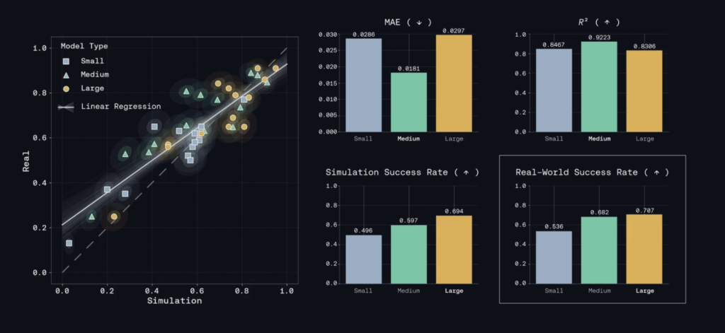
Genesis AI released Genesis World 1.0. The platform consists of four components: the Genesis World physics engine, Nyx (a real-time path-traced renderer), Quadrants (a Python-to-GPU compiler), and a simulation interface. It is designed to accelerate robotics foundation model development through simulation-based evaluation. Robotics model development has two bottlenecks: data and iteration speed. The field has focused heavily on data. Genesis AI argues the slower, less-discussed bottleneck is the model development cycle itself — specifically, how fast teams can evaluate candidate policies and compare model checkpoints. What Problem Does This Solve? A typical policy evaluation at Genesis spans hundreds of tasks with hundreds of episodes each. Running that in the real world requires more than 200 hours of continuous robot operation with one operator and one robot station — for a single evaluation pass. Statistically meaningful comparisons across checkpoints require many such passes. Genesis World 1.0 runs the same evaluation in under 0.5 hours, with no human or hardware in the loop and bit-exact result consistency across runs. That is roughly two orders of magnitude faster than real-world evaluation. The research team deliberately chose to prioritize evaluation before using simulation for training data generation. Their reasoning: if training and evaluation share the same simulated distribution, a performance improvement could reflect a tighter fit to simulator dynamics rather than a genuinely better model. Keeping the two pipelines separated produces a cleaner signal. The research team describes this evaluation approach as zero-shot real-to-sim: policies evaluated in simulation are trained exclusively on real-world data. No simulated data enters pretraining. Sim-to-Real Correlation Results Genesis research team reports a Pearson correlation of 0.8996 (95% CI: [0.7439, 0.9314]) between simulation and on-hardware rollouts. The evaluation covered three model variants (Small, Medium, Large) across 14 tasks with 200 episodes per task. The research team ran 1,000,000 bootstrap iterations to estimate confidence intervals. The Mean Maximum Rank Violation (MMRV) — a metric proposed in SimplerEnv — was 0.0166 (95% CI: [0.0102, 0.0474]). A low MMRV means the simulator preserves the relative performance ranking of different models. To diagnose where sim-to-real divergence comes from, Genesis team built a real-time side-by-side rig. It runs the simulator and physical robot in parallel from the same initialization. Observations — camera frames and proprioception — can come from the simulator, the robot, or a blend of both. Swapping one source at a time isolates whether divergence originates from physics, rendering, communication, or control. After this work, their reality gap is 45% smaller, measured by FID score on their dataset, than the next-best alternative simulator. https://www.genesis.ai/blog/the-role-of-simulation-in-scalable-robotics-genesis-world-10-and-the-path-forward?x_refresh=1 The Four Components of Genesis World 1.0 Nyx — Real-Time Path-Traced Rendering Nyx is a GPU-accelerated path tracer that plugs into Genesis World as a camera sensor. It is available as the gs-nyx-plugin Python package. Prebuilt wheels are available for x86-64 Linux (manylinux 2.34+) and Windows 10/11, and require an NVIDIA GPU with CUDA. Nyx targets noise-free 1080p frames in 4 ms or less on a high-end consumer GPU, with no baking and no ghosting. To reach that target, it uses a visibility buffer, a bindless GPU-driven architecture, MSAA, hardware ray tracing, hardware matrix cores, and video compression. Path tracing is the baseline: multi-bounce lighting, soft shadows, and indirect illumination are correct by construction. A physically grounded camera model sits on top. An HDRI pipeline lights scenes with measured radiance. Assets come from internal scanning and photogrammetry. 3D Gaussian splats extend coverage where mesh reconstruction is insufficient. Nyx is driven by batched physics rather than scene-by-scene execution. This allows thousands of parallel rollouts — each with its own scenario, lighting, and camera trajectory — to pass through a single unified rendering pipeline. Genesis World Physics — Unified Multi-Physics Engine The Genesis World physics platform is open source (Apache 2.0) and runs multi-physics in a single pipeline: articulated rigid bodies (MJCF/URDF/USD), FEM for elastic deformables and cloth, MPM for granular and elasto-plastic materials, SPH for fluids, and PBD for fast cloth and position-based liquids. Three interchangeable couplers are available behind the same scene API: a fast general-purpose coupler; a Drake-style Semi-Analytic Primal coupler with hydroelastic contact; and an Incremental Potential Contact (IPC) coupler for intersection-free contact in deformable scenes. Switching between couplers requires a one-line code change, with no changes to assets, sensors, or the policy interface. Genesis World 1.0 introduced two new solvers. The External Articulation Constraint (built on top of libuipc) embeds joint-space dynamics directly into IPC’s optimization, so joint-space forces and contact forces resolve simultaneously rather than staggered across separate solvers. The second is barrier-free elastodynamics, which replaces IPC’s logarithmic barrier with a custom augmented Lagrangian. Standard IPC’s barrier makes the Hessian ill-conditioned as contacts tighten. The augmented Lagrangian formulation avoids this, allowing every contact pair returned by continuous collision detection to enter the active set immediately. The research team reports up to 103× faster performance than traditional IPC in contact-heavy scenes, with intersection-free guarantees maintained. Additional improvements: new sensors (point-cloud tactile, temperature-grid, proximity), Implicit FEM with Newton + CG solver, and expanded asset support (URDF xacro, MuJoCo general actuators, compound/mimic joints, equality/weld constraints). Quadrants — Python-to-GPU Compiler Quadrants is a cross-platform compiler for GPU-accelerated physics simulation, developed by Genesis AI and released under Apache 2.0. Kernels are written in plain Python and JIT-compiled to NVIDIA CUDA, AMD ROCm, Apple Metal, Vulkan, and x86/ARM64 CPUs via LLVM. It was forked from Taichi in June 2025. The name references the Chinese philosophical saying that Taichi gives rise to the Four Forms (Quadrants). Key performance improvements over upstream Taichi: up to 4.6× faster runtime on Genesis manipulation and locomotion benchmarks. Warm-cache startup time for single_franka_envs.py dropped from 7.2 seconds to 0.3 seconds — a more than 10× speedup. Reverse-mode autodiff is now a first-class citizen on all backends, making differentiable simulation portable. Physics steps are recorded as single kernel graphs, removing per-step launch latency. Independent kernels run in parallel via streams. Dense linear algebra (Cholesky factorization, triangular solves) compiles to 16×16 tile-blocked code paths. A perf-dispatch layer benchmarks kernel variants on first call and caches the fastest choice

Genesis AI Releases Nyx, Quadrants, and Genesis World 1.0 Physics Platform for Scalable Robotics Foundation Model Evaluation Read Post »

AI, Committee, 新闻, Uncategorized

SSDAU: Structured Semantic Data Augmentation for Joint Entity and Relation Extraction

arXiv:2605.23440v4 Announce Type: replace Abstract: Joint Entity and Relation Extraction (JERE) is highly sensitive to training data quality, making data augmentation a natural way to improve generalization. However, existing augmentation methods often weaken entity relevance and disrupt semantic structure, limiting their effectiveness for JERE. In this paper, we propose textbf{Structured Semantic Data Augmentation (SSDAU)}, a method designed to preserve triple-aware semantic structure during augmentation. SSDAU segments text by entity labels, captures semantic features through context-aware encoding, and restructures entity semantics to generate augmented data. To distinguish semantically similar entities, SSDAU combines contextualized embeddings with traditional similarity scores. To reduce topic inconsistency, we apply BERTopic-based filtering to remove irrelevant augmentations. We evaluate SSDAU on datasets with different annotation types and compare its performance on five representative JERE models against seven popular augmentation baselines. Experiments show that SSDAU generates semantically consistent data, is more robust to ambiguity than non-LLM methods (8.95% vs. 23.58% average relative F1 decrease), and significantly outperforms strong alternatives in most settings.

SSDAU: Structured Semantic Data Augmentation for Joint Entity and Relation Extraction Read Post »

AI, Committee, 新闻, Uncategorized

The deadly Ebola outbreak is proving difficult to control

The alert was raised on May 5. Four health-care workers in the Ituri Province of the Democratic Republic of the Congo had died from an unknown illness within four days. Rapid response teams were sent to investigate, and tests at a research center in Kinshasa revealed the culprit: the Bundibugyo virus, one of the viruses that cause Ebola. Suspected cases of the disease have snowballed in the last few weeks. By May 24, the WHO had estimated that 223 people had died from the disease. There were over 900 suspected cases. Today’s figures are likely to be higher. A couple of weeks ago, I covered the hantavirus outbreak aboard a cruise ship. Three people sadly died, but the outbreak itself was kept under control. There have been no further deaths, and passengers have been safely repatriated. The picture for Ebola is far bleaker. And there are several reasons why. The most obvious is the disease itself. Ebola is a severe disease with an average 50% fatality rate. Previous outbreaks have resulted in thousands of deaths. (Hantavirus also has a high fatality rate, but it doesn’t usually spread as easily between humans.)  Between 2014 and 2016, an Ebola outbreak in West Africa caused more than 11,000 deaths. A more recent outbreak, which took place between 2018 and 2020, caused 2,299 deaths before being brought under control with a vaccination campaign. But those outbreaks were caused by the Zaire virus, which has a different genetic sequence. There is no vaccine for the Bundibugyo virus. We don’t know if the two vaccines approved for Zaire might also work for Bundibugyo. There’s a concern they might even make things worse by interfering with a person’s immune response to the virus.   Scientists are working on potential Bundibugyo vaccines. But the most advanced efforts are still months away from clinical trials. There are no specific antiviral treatments for the virus, either. So to control the outbreak, health-care workers are trying to stop the spread of the disease. Ebolaviruses can be transmitted to humans by animals including fruit bats, chimpanzees, and gorillas. They can then spread between people via contact with bodily fluids such as blood or vomit. That’s why the virus is often spread among family members, to health-care workers, and during some burial services. The WHO advises isolating people who have the virus in treatment centers. It also recommends safe burial measures that limit physical contact with the deceased, for example. Communities need to be informed about the virus and how it spreads, and health professionals should be on hand to diagnose cases and track them. That’s all easier said than done in an era of misinformation. Some members of the community even doubt whether the disease is real. There have been three attacks on health-care facilities in the region in recent weeks. Last week, two treatment centers were burned down. The first incident occurred after relatives of a deceased man were prohibited from retrieving his (infectious) body. As a result of the second incident, 18 suspected cases reentered the community. A couple of days later, a group of men unleashed gunfire at Mongbwalu General Hospital, which was also treating people with Ebola. They were demanding the bodies of their deceased relatives. There are more causes for concern when it comes to the spread of the virus. The Ebola outbreak is thought to have originated in Mongbwalu, a high-traffic mining hub. People who caught the virus in Mongbwalu are thought to have sought care in neighboring districts. And the wider province borders both South Sudan and Uganda. So far, Uganda has reported seven confirmed cases and one death. South Sudan’s health ministry has said it will strengthen surveillance, but no cases have been reported in the country so far.  Violence in the region is making it much harder to contain the spread of the virus, too. Conflict involving multiple armed groups, including deadly attacks on civilians, has hampered humanitarian and health-care efforts. Poor infrastructure and damaged roads make matters even worse. Food insecurity is ravaging the region as well—this year, nearly 10 million people in the region face acute hunger. Together, these factors are making it “nearly impossible” to isolate people with Ebola and trace others who have been in contact with them, WHO director general Tedros Adhanom Ghebreyesus said in a statement earlier this week. The dismantling of US aid programs hasn’t helped either. US government funding for international health projects has steeply declined since the start of President Donald Trump’s second term. These cuts have harmed disease surveillance systems, according to the International Rescue Committee, a humanitarian nonprofit. “Funding cuts have left the region dangerously exposed,” Heather Reoch Kerr, the organization’s country director for the Democratic Republic of the Congo, said in a statement. “Years of underinvestment and recent funding cuts have left many health facilities without adequate protective equipment, surveillance capacity, or frontline support needed to respond quickly and safely.” The US has mobilized emergency funding for the outbreak, and a spokesperson for the State Department has argued that none of the administration’s actions have hampered the Ebola response. But health experts counter that the damage has already been done. On May 17, the WHO declared the Ebola outbreak a public health emergency of international concern. In a statement on Wednesday, Tedros described the situation as “a catastrophic collision of disease and conflict with the Ebola outbreak in Ituri province outpacing the response.”In an online appeal to residents on Wednesday, ahead of an in-person visit, Tedros pleaded for a ceasefire and commended the spirit of community members. He also acknowledged the steep challenges they face. “You are already carrying so much: malaria, hunger, insecurity, and the daily struggle to keep your families safe,” he wrote in French. “And now Ebola. It’s not fair, and I won’t pretend otherwise.” This article first appeared in The Checkup, MIT Technology Review’s weekly biotech newsletter. To receive it in your inbox every Thursday, and read articles like this first, sign up here.

The deadly Ebola outbreak is proving difficult to control Read Post »

AI, Committee, 新闻, Uncategorized

How the Pope’s Magnifica Humanitas offers a template for individuals to meet the AI moment

Pope Leo XIV’s new encyclical on artificial intelligence includes a statement that warrants serious attention from technologists and policymakers: “Technology is never neutral.” Magnifica Humanitas (“Magnificent Humanity”) is a clarion call to all people to act with courage and solidarity as we enter an age already being transformed by artificial intelligence, the greatest change in human life since the Industrial Revolution. As the pope says, the choice before us—the choice AI presents—is one between the Tower of Babel and the rebuilding of our common humanity.  In the biblical story of the Tower of Babel, humans sought to build a massive structure that reached all the way to Heaven, only to have their project thwarted when God made those involved unable to understand one another. It was a pursuit fixated on relentless growth, divorced from any concern about God’s commandments or the human cost. It resulted in failure and atomization. The Book of Nehemiah, however, offers a contrasting narrative, in which the rebuilding of Jerusalem after a period of violence and displacement becomes an opportunity for humanity to show its collaborative resilience. As the encyclical puts it, “The city is reborn, not through the initiative of one man, but through the shared responsibility of all: men, women, priests, artisans, heads of households and young people all play a part. It is an undertaking with God at the center, which rebuilds relationships before rebuilding with stones.”  Is there any question which road we are currently barreling down? And can there be any doubt which we would do well to walk together?  We are both Catholics, members of religious communities and longtime advocates within the movement for socially responsible investment. Of particular interest to us and that movement is Pope Leo’s point that AI is not some force of nature or hyperrational, ineffable entity. Instead, he reminds us, AI is ultimately another commercial product, one emerging at a point in history when excessive power over commerce and the wider society has amassed in a vanishingly small number of hands.  It’s a powerful message. It’s also one that institutional investors have been acting on for years. This encyclical doesn’t break new ground so much as ratify a governance effort that’s already underway, led not by states or international bodies but by shareholders. When governments fail to meaningfully regulate, and corporations cannot be trusted to do what is beneficial beyond their own bottom line, people in society still have the power to set us on the right path, and indeed have the duty to do so.  Around the world, AI systems are being deployed at scale with remarkably little institutional oversight. There is no AI safety board. The US Federal Trade Commission has jurisdiction over unfair practices but limited authority over algorithmic design. The National Institute of Standards and Technology publishes guidance that most companies ignore. The EU AI Act is partially in force but addresses only a sliver of the deployment surface. Institutional investors have stepped into this vacuum. Coalitions including the membership of the Interfaith Center on Corporate Responsibility, representing investors managing over $400 billion in assets, have spent the past several proxy seasons filing resolutions demanding transparency, risk assessment, and accountability around AI deployment. Secular institutional investors have joined them, treating AI governance failures as material business risks. Shareholders have called tech giants including Alphabet, Amazon, Nvidia, Palantir, and Uber to account and demanded that AI not be used for acts of violence or other violations of human rights. The importance of this aspect of corporate governance was highlighted tragically in the opening hours of the war against Iran, when AI was used to help identify targets for thousands of missile strikes that killed hundreds of people.   Investors have also challenged executives at CVS and UnitedHealth Group to ensure that AI not be used to undermine the well-being of patients and quality of health care across the United States.  At companies including Meta and Microsoft, shareholders have decried the environmental impact of AI data centers, which consume vast amounts of energy and precious water resources, and in turn can emit large amounts of greenhouse gases.  Within creative industries, investors have challenged the leadership at companies like Disney, Netflix, and Warner Bros. to demand transparency about the ways they are using AI and to defend the inimitable human element in storytelling.  Soon, with OpenAI, Anthropic, and Grok all set to enter the public markets, we will be able to exert similar influence over what are now all privately held entities. These actions by concerned investors not only call out misdeeds but hold fast to an immutable truth: that it is wrong to use technology to kill, harm, or oppress people. Every human being has a right to safe and effective health care and the opportunity to earn a dignified living. The stories we tell each other matter and require the human creative spark.  Investor advocates hail from a range of faith traditions. Some have no formal religious faith. Yet in their informed and tenacious advocacy, all these people echo the calls embedded within Pope Leo’s encyclical and act on its declaration that “it is essential that the use of AI, especially when it touches on public goods and fundamental rights, be guided by clear criteria and effective oversight.”  Encyclicals mark time. A century from now, how will we be remembered for how we met this moment? Will we be seen as having been too timid or shortsighted to prevent a small group of unfathomably wealthy and self-interested people from seizing ever greater control over the human family’s shared destiny?  Or will the years ahead be remembered as a turning point that helped us rebuild our common humanity? Let this be a time when people of good will and diverse talents come together through their own magnificent humanity to build a future that honors our Creator. Father Séamus Finn, OMI, is a global leader in faith-based and socially responsible investing and a priest of the Oblates of Mary Immaculate, a missionary religious congregation.

How the Pope’s Magnifica Humanitas offers a template for individuals to meet the AI moment Read Post »

We use cookies to improve your experience and performance on our website. You can learn more at 隱私權政策 and manage your privacy settings by clicking Settings.

Privacy Preferences

You can choose your cookie settings by turning on/off each type of cookie as you wish, except for essential cookies.

Allow All
Manage Consent Preferences
  • Always Active

Save
zh_CN