YouZum

Uncategorized

AI, Committee, Nachrichten, Uncategorized

Investigating Gender Stereotypes in Large Language Models via Social Determinants of Health

arXiv:2603.09416v1 Announce Type: new Abstract: Large Language Models (LLMs) excel in Natural Language Processing (NLP) tasks, but they often propagate biases embedded in their training data, which is potentially impactful in sensitive domains like healthcare. While existing benchmarks evaluate biases related to individual social determinants of health (SDoH) such as gender or ethnicity, they often overlook interactions between these factors and lack context-specific assessments. This study investigates bias in LLMs by probing the relationships between gender and other SDoH in French patient records. Through a series of experiments, we found that embedded stereotypes can be probed using SDoH input and that LLMs rely on embedded stereotypes to make gendered decisions, suggesting that evaluating interactions among SDoH factors could usefully complement existing approaches to assessing LLM performance and bias.

Investigating Gender Stereotypes in Large Language Models via Social Determinants of Health Beitrag lesen »

AI, Committee, Nachrichten, Uncategorized

Fish Audio Releases Fish Audio S2: A New Generation of Expressive Text-to-Speech (TTS) with Absurdly Controllable Emotion

The landscape of Text-to-Speech (TTS) is moving away from modular pipelines toward integrated Large Audio Models (LAMs). Fish Audio’s release of S2-Pro, the flagship model within the Fish Speech ecosystem, represents a shift toward open architectures capable of high-fidelity, multi-speaker synthesis with sub-150ms latency. The release provides a framework for zero-shot voice cloning and granular emotional control using a Dual-Auto-Regressive (AR) approach. Architecture: The Dual-AR Framework and RVQ The fundamental technical distinction in Fish Audio S2-Pro is its hierarchical Dual-AR architecture. Traditional TTS models often struggle with the trade-off between sequence length and acoustic detail. S2-Pro addresses this by bifurcating the generation process into two specialized stages: a ‘Slow AR’ model and a ‘Fast AR’ model. The Slow AR Model (4B Parameters): This component operates on the time-axis. It is responsible for processing linguistic input and generating semantic tokens. By utilizing a larger parameter count (approximately 4 billion), the Slow AR model captures long-range dependencies, prosody, and the structural nuances of speech. The Fast AR Model (400M Parameters): This component processes the acoustic dimension. It predicts the residual codebooks for each semantic token. This smaller, faster model ensures that the high-frequency details of the audio—timbre, breathiness, and texture—are generated with high efficiency. This system relies on Residual Vector Quantization (RVQ). In this setup, raw audio is compressed into discrete tokens across multiple layers (codebooks). The first layer captures the primary acoustic features, while subsequent layers capture the ‘residuals’ or the remaining errors from the previous layer. This allows the model to reconstruct high-fidelity 44.1kHz audio while maintaining a manageable token count for the Transformer architecture. Emotional Control via In-Context Learning and Inline Tags Fish Audio S2-Pro achieves what the developers describe as ‘absurdly controllable emotion’ through two primary mechanisms: zero-shot in-context learning and natural language inline control. In-Context Learning (ICL): Unlike older generations of TTS that required explicit fine-tuning to mimic a specific voice, S2-Pro utilizes the Transformer’s ability to perform in-context learning. By providing a reference audio clip—ideally between 10 and 30 seconds—the model extracts the speaker’s identity and emotional state. The model treats this reference as a prefix in its context window, allowing it to continue the “sequence” in the same voice and style. Inline Control Tags: The model supports dynamic emotional transitions within a single generation pass. Because the model was trained on data containing descriptive linguistic markers, developers can insert natural language tags directly into the text prompt. For example: [whisper] I have a secret [laugh] that I cannot tell you. The model interprets these tags as instructions to modify the acoustic tokens in real-time, adjusting pitch, intensity, and rhythm without requiring a separate emotional embedding or external control vector. Performance Benchmarks and SGLang Integration Integrating TTS into real-time applications, the primary constraint is ‘Time to First Audio’ (TTFA). Fish Audio S2-Pro is optimized for a sub-150ms latency, with benchmarks on NVIDIA H200 hardware reaching approximately 100ms. Several technical optimizations contribute to this performance: SGLang and RadixAttention: S2-Pro is designed to work with SGLang, a high-performance serving framework. It utilizes RadixAttention, which allows for efficient Key-Value (KV) cache management. In a production environment where the same “master” voice prompt (reference clip) is used repeatedly, RadixAttention caches the prefix’s KV states. This eliminates the need to re-compute the reference audio for every request, significantly reducing the prefill time. Multi-Speaker Single-Pass Generation: The architecture allows for multiple speaker identities to be present within the same context window. This permits the generation of complex dialogues or multi-character narrations in a single inference call, avoiding the latency overhead of switching models or reloading weights for different speakers. Technical Implementation and Data Scaling The Fish Speech repository provides a Python-based implementation utilizing PyTorch. The model was trained on a diverse dataset comprising over 300,000 hours of multi-lingual audio. This scale is what enables the model’s robust performance across different languages and its ability to handle ‘non-verbal’ vocalizations like sighs or hesitations. The training pipeline involves: VQ-GAN Training: Training the quantizer to map audio into a discrete latent space. LLM Training: Training the Dual-AR transformers to predict those latent tokens based on text and acoustic prefixes. The VQ-GAN used in S2-Pro is specifically tuned to minimize artifacts during the decoding process, ensuring that even at high compression ratios, the reconstructed audio remains ‘transparent’ (indistinguishable from the source to the human ear). Key Takeaways Dual-AR Architecture (Slow/Fast): Unlike single-stage models, S2-Pro splits tasks between a 4B parameter ‘Slow AR’ model (for linguistic and prosodic structure) and a 400M parameter ‘Fast AR’ model (for acoustic refinement), optimizing both detail and speed. Sub-150ms Latency: Engineered for real-time conversational AI, the model achieves a Time-to-First-Audio (TTFA) of ~100ms on high-end hardware, making it suitable for live agents and interactive applications. Hierarchical RVQ Encoding: By using Residual Vector Quantization, the system compresses 44.1kHz audio into discrete tokens across multiple layers. This allows the model to reconstruct complex vocal textures—including breaths and sighs—without the computational bloat of raw waveforms. Zero-Shot In-Context Learning: Developers can clone a voice and its emotional state by providing a 10–30 second reference clip. The model treats this as a prefix, adopting the speaker’s timbre and prosody without requiring additional fine-tuning. RadixAttention & SGLang Integration: Optimized for production, S2-Pro leverages RadixAttention to cache KV states of voice prompts. This allows for nearly instant generation when using the same speaker repeatedly, drastically reducing prefill overhead. Check out Model Card and Repo. Also, feel free to follow us on Twitter and don’t forget to join our 120k+ ML SubReddit and Subscribe to our Newsletter. Wait! are you on telegram? now you can join us on telegram as well. The post Fish Audio Releases Fish Audio S2: A New Generation of Expressive Text-to-Speech (TTS) with Absurdly Controllable Emotion appeared first on MarkTechPost.

Fish Audio Releases Fish Audio S2: A New Generation of Expressive Text-to-Speech (TTS) with Absurdly Controllable Emotion Beitrag lesen »

AI, Committee, Nachrichten, Uncategorized

Google AI Introduces Gemini Embedding 2: A Multimodal Embedding Model that Lets Your Bring Text, Images, Video, Audio, and Docs into the Embedding Space

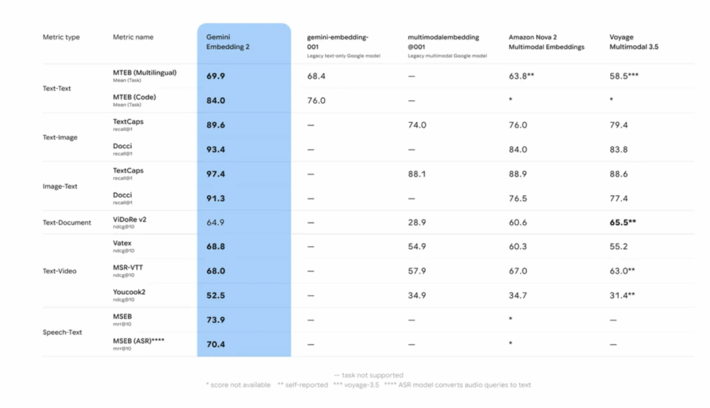
Google expanded its Gemini model family with the release of Gemini Embedding 2. This second-generation model succeeds the text-only gemini-embedding-001 and is designed specifically to address the high-dimensional storage and cross-modal retrieval challenges faced by AI developers building production-grade Retrieval-Augmented Generation (RAG) systems. The Gemini Embedding 2 release marks a significant technical shift in how embedding models are architected, moving away from modality-specific pipelines toward a unified, natively multimodal latent space. Native Multimodality and Interleaved Inputs The primary architectural advancement in Gemini Embedding 2 is its ability to map five distinct media types—Text, Image, Video, Audio, and PDF—into a single, high-dimensional vector space. This eliminates the need for complex pipelines that previously required separate models for different data types, such as CLIP for images and BERT-based models for text. The model supports interleaved inputs, allowing developers to combine different modalities in a single embedding request. This is particularly relevant for use cases where text alone does not provide sufficient context. The technical limits for these inputs are defined as: Text: Up to 8,192 tokens per request. Images: Up to 6 images (PNG, JPEG, WebP, HEIC/HEIF). Video: Up to 120 seconds of video (MP4, MOV, etc.). Audio: Up to 80 seconds of native audio (MP3, WAV, etc.) without requiring a separate transcription step. Documents: Up to 6 pages of PDF files. By processing these inputs natively, Gemini Embedding 2 captures the semantic relationships between a visual frame in a video and the spoken dialogue in an audio track, projecting them as a single vector that can be compared against text queries using standard distance metrics like Cosine Similarity. Efficiency via Matryoshka Representation Learning (MRL) Storage and compute costs are often the primary bottlenecks in large-scale vector search. To mitigate this, Gemini Embedding 2 implements Matryoshka Representation Learning (MRL). Standard embedding models distribute semantic information evenly across all dimensions. If a developer truncates a 3,072-dimension vector to 768 dimensions, the accuracy typically collapses because the information is lost. In contrast, Gemini Embedding 2 is trained to pack the most critical semantic information into the earliest dimensions of the vector. The model defaults to 3,072 dimensions, but Google team has optimized three specific tiers for production use: 3,072: Maximum precision for complex legal, medical, or technical datasets. 1,536: A balance of performance and storage efficiency. 768: Optimized for low-latency retrieval and reduced memory footprint. Matryoshka Representation Learning (MRL) enables a ‘short-listing’ architecture. A system can perform a coarse, high-speed search across millions of items using the 768-dimension sub-vectors, then perform a precise re-ranking of the top results using the full 3,072-dimension embeddings. This reduces the computational overhead of the initial retrieval stage without sacrificing the final accuracy of the RAG pipeline. Benchmarking: MTEB and Long-Context Retrieval Google AI’s internal evaluation and performance on the Massive Text Embedding Benchmark (MTEB) indicate that Gemini Embedding 2 outperforms its predecessor in two specific areas: Retrieval Accuracy and Robustness to Domain Shift. Many embedding models suffer from ‘domain drift,’ where accuracy drops when moving from generic training data (like Wikipedia) to specialized domains (like proprietary codebases). Gemini Embedding 2 utilized a multi-stage training process involving diverse datasets to ensure higher zero-shot performance across specialized tasks. The model’s 8,192-token window is a critical specification for RAG. It allows for the embedding of larger ‘chunks’ of text, which preserves the context necessary for resolving coreferences and long-range dependencies within a document. This reduces the likelihood of ‘context fragmentation,’ a common issue where a retrieved chunk lacks the information needed for the LLM to generate a coherent answer. https://blog.google/innovation-and-ai/models-and-research/gemini-models/gemini-embedding-2/ Key Takeaways Native Multimodality: Gemini Embedding 2 supports five distinct media types—Text, Image, Video, Audio, and PDF—within a unified vector space. This allows for interleaved inputs (e.g., an image combined with a text caption) to be processed as a single embedding without separate model pipelines. Matryoshka Representation Learning (MRL): The model is architected to store the most critical semantic information in the early dimensions of a vector. While it defaults to 3,072 dimensions, it supports efficient truncation to 1,536 or 768 dimensions with minimal loss in accuracy, reducing storage costs and increasing retrieval speed. Expanded Context and Performance: The model features an 8,192-token input window, allowing for larger text ‘chunks’ in RAG pipelines. It shows significant performance improvements on the Massive Text Embedding Benchmark (MTEB), specifically in retrieval accuracy and handling specialized domains like code or technical documentation. Task-Specific Optimization: Developers can use task_type parameters (such as RETRIEVAL_QUERY, RETRIEVAL_DOCUMENT, or CLASSIFICATION) to provide hints to the model. This optimizes the vector’s mathematical properties for the specific operation, improving the “hit rate” in semantic search. Check out Technical details, in Public Preview via the Gemini API and Vertex AI. Also, feel free to follow us on Twitter and don’t forget to join our 120k+ ML SubReddit and Subscribe to our Newsletter. Wait! are you on telegram? now you can join us on telegram as well. The post Google AI Introduces Gemini Embedding 2: A Multimodal Embedding Model that Lets Your Bring Text, Images, Video, Audio, and Docs into the Embedding Space appeared first on MarkTechPost.

Google AI Introduces Gemini Embedding 2: A Multimodal Embedding Model that Lets Your Bring Text, Images, Video, Audio, and Docs into the Embedding Space Beitrag lesen »

AI, Committee, Nachrichten, Uncategorized

QuadAI at SemEval-2026 Task 3: Ensemble Learning of Hybrid RoBERTa and LLMs for Dimensional Aspect-Based Sentiment Analysis

arXiv:2603.07766v1 Announce Type: new Abstract: We present our system for SemEval-2026 Task 3 on dimensional aspect-based sentiment regression. Our approach combines a hybrid RoBERTa encoder, which jointly predicts sentiment using regression and discretized classification heads, with large language models (LLMs) via prediction-level ensemble learning. The hybrid encoder improves prediction stability by combining continuous and discretized sentiment representations. We further explore in-context learning with LLMs and ridge-regression stacking to combine encoder and LLM predictions. Experimental results on the development set show that ensemble learning significantly improves performance over individual models, achieving substantial reductions in RMSE and improvements in correlation scores. Our findings demonstrate the complementary strengths of encoder-based and LLM-based approaches for dimensional sentiment analysis. Our development code and resources will be shared at https://github.com/aaronlifenghan/ABSentiment

QuadAI at SemEval-2026 Task 3: Ensemble Learning of Hybrid RoBERTa and LLMs for Dimensional Aspect-Based Sentiment Analysis Beitrag lesen »

AI, Committee, Nachrichten, Uncategorized

SynPlanResearch-R1: Encouraging Tool Exploration for Deep Research with Synthetic Plans

arXiv:2603.07853v1 Announce Type: cross Abstract: Research Agents enable models to gather information from the web using tools to answer user queries, requiring them to dynamically interleave internal reasoning with tool use. While such capabilities can in principle be learned via reinforcement learning with verifiable rewards (RLVR), we observe that agents often exhibit poor exploration behaviors, including premature termination and biased tool usage. As a result, RLVR alone yields limited improvements. We propose SynPlanResearch-R1, a framework that synthesizes tool-use trajectories that encourage deeper exploration to shape exploration during cold-start supervised fine-tuning, providing a strong initialization for subsequent RL. Across seven multi-hop and open-web benchmarks, framework improves performance by up to 6.0% on Qwen3-8B and 5.8% on Qwen3-4B backbones respectively compared to SOTA baselines. Further analyses of tool-use patterns and training dynamics compared to baselines shed light on the factors underlying these gains. Our code is publicly available at https://github.com/HansiZeng/syn-plan-research.

SynPlanResearch-R1: Encouraging Tool Exploration for Deep Research with Synthetic Plans Beitrag lesen »

AI, Committee, Nachrichten, Uncategorized

Whitening Reveals Cluster Commitment as the Geometric Separator of Hallucination Types

arXiv:2603.07755v1 Announce Type: new Abstract: A geometric hallucination taxonomy distinguishes three failure types — center-drift (Type~1), wrong-well convergence (Type~2), and coverage gaps (Type~3) — by their signatures in embedding cluster space. Prior work found Types~1 and~2 indistinguishable in full-dimensional contextual measurement. We address this through PCA-whitening and eigenspectrum decomposition on GPT-2-small, using multi-run stability analysis (20 seeds) with prompt-level aggregation. Whitening transforms the micro-signal regime into a space where peak cluster alignment (max_sim) separates Type~2 from Type~3 at Holm-corrected significance, with condition means following the taxonomy’s predicted ordering: Type~2 (highest commitment) $>$ Type~1 (intermediate) $>$ Type~3 (lowest). A first directionally stable but underpowered hint of Type~1/2 separation emerges via the same metric, generating a capacity prediction for larger models. Prompt diversification from 15 to 30 prompts per group eliminates a false positive in whitened entropy that appeared robust at the smaller set, demonstrating prompt-set sensitivity in the micro-signal regime. Eigenspectrum decomposition localizes this artifact to the dominant principal components and confirms that Type~1/2 separation does not emerge in any spectral band, rejecting the spectral mixing hypothesis. The contribution is threefold: whitening as preprocessing that reveals cluster commitment as the theoretically correct separating metric, evidence that the Type~1/2 boundary is a capacity limitation rather than a measurement artifact, and a methodological finding about prompt-set fragility in near-saturated representation spaces.

Whitening Reveals Cluster Commitment as the Geometric Separator of Hallucination Types Beitrag lesen »

AI, Committee, Nachrichten, Uncategorized

Jr. AI Scientist and Its Risk Report: Autonomous Scientific Exploration from a Baseline Paper

arXiv:2511.04583v3 Announce Type: replace-cross Abstract: Understanding the current capabilities and risks of AI Scientist systems is essential for ensuring trustworthy and sustainable AI-driven scientific progress while preserving the integrity of the academic ecosystem. To this end, we develop Jr. AI Scientist, a state-of-the-art autonomous AI scientist system that mimics the core research workflow of a novice student researcher: Given the baseline paper from the human mentor, it analyzes its limitations, formulates novel hypotheses for improvement, validates them through rigorous experimentation, and writes a paper with the results. Unlike previous approaches that assume full automation or operate on small-scale code, Jr. AI Scientist follows a well-defined research workflow and leverages modern coding agents to handle complex, multi-file implementations, leading to scientifically valuable contributions. Through our experiments, the Jr. AI Scientist successfully generated new research papers that build upon real NeurIPS, IJCV, and ICLR works by proposing and implementing novel algorithms. For evaluation, we conducted automated assessments using AI Reviewers, author-led evaluations, and submissions to Agents4Science, a venue dedicated to AI-driven scientific contributions. The findings demonstrate that Jr. AI Scientist generates papers receiving higher review scores by DeepReviewer than existing fully automated systems. Nevertheless, we identify important limitations from both the author evaluation and the Agents4Science reviews, indicating the potential risks of directly applying current AI Scientist systems and key challenges for future research. Finally, we comprehensively report various risks identified during development. We believe this study clarifies the current role and limitations of AI Scientist systems, offering insights into the areas that still require human expertise and the risks that may emerge as these systems evolve.

Jr. AI Scientist and Its Risk Report: Autonomous Scientific Exploration from a Baseline Paper Beitrag lesen »

AI, Committee, Nachrichten, Uncategorized

The ‘Bayesian’ Upgrade: Why Google AI’s New Teaching Method is the Key to LLM Reasoning

Large Language Models (LLMs) are the world’s best mimics, but when it comes to the cold, hard logic of updating beliefs based on new evidence, they are surprisingly stubborn. A team of researchers from Google argue that the current crop of AI agents falls far short of ‘probabilistic reasoning’—the ability to maintain and update a ‘world model’ as new information trickles in. The solution? Stop trying to give them the right answers and start teaching them how to guess like a mathematician. The Problem: The ‘One-and-Done’ Plateau While LLMs like Gemini-1.5 Pro and GPT-4.1 Mini can write code or summarize emails, they struggle as interactive agents. Imagine a flight booking assistant: it needs to infer your preferences (price vs. duration) by watching which flights you pick over several rounds. The research team found that off-the-shelf LLMs—including heavyweights like Llama-3-70B and Qwen-2.5-32B—showed ‘little or no improvement’ after the first round of interaction. While a ‘Bayesian Assistant’ (a symbolic model using Bayes’ rule) gets more accurate with every data point, standard LLMs plateaued almost immediately, failing to adapt their internal ‘beliefs’ to the user’s specific reward function. Meet Bayesian Teaching The research team introduced a technique called Bayesian Teaching. Instead of fine-tuning a model on ‘correct’ data (what they call an Oracle Teacher), they fine-tuned it to mimic a Bayesian Assistant—a model that explicitly uses Bayes’ rule to update a probability distribution over possible user preferences. Here is the technical breakdown: The Task: A five-round flight recommendation interaction. Flights are defined by features like price, duration, and stops. The Reward Function: A vector representing user preferences (e.g., a strong preference for low prices). The Posterior Update: After each round, the Bayesian Assistant updates its posterior distribution based on the prior (initial assumptions) and the likelihood (the probability the user would pick a certain flight given a specific reward function). By using Supervised Fine-Tuning (SFT) on these Bayesian interactions, the research team forced the LLMs to adopt the process of reasoning under uncertainty, not just the final result. Why ‘Educated Guesses’ Beat Correct Answers The most counter-intuitive finding of the research is that Bayesian Teaching consistently outperformed Oracle Teaching. In ‘Oracle Teaching,’ the model is trained on a teacher that already knows exactly what the user wants. In ‘Bayesian Teaching,’ the teacher is often wrong in early rounds because it is still learning. However, those ‘educated guesses’ provide a much stronger learning signal. By watching the Bayesian Assistant struggle with uncertainty and then update its beliefs after receiving feedback, the LLM learns the ‘skill’ of belief updating. The results were stark: Bayesian-tuned models (like Gemma-2-9B or Llama-3-8B) were not only more accurate but agreed with the ‘gold standard’ Bayesian strategy roughly 80% of the time—significantly higher than their original versions. Generalization: Beyond Flights to Web Shopping For devs, the ‘holy grail’ is generalization. A model trained on flight data shouldn’t just be good at flights; it should understand the concept of learning from a user. The research team tested their fine-tuned models on: Increased Complexity: Moving from four flight features to eight. New Domains: Hotel recommendations. Real-World Scenarios: A web shopping task using real products (titles and descriptions) from a simulated environment. Even though the models were only fine-tuned on synthetic flight data, they successfully transferred those probabilistic reasoning skills to hotel booking and web shopping. In fact, the Bayesian LLMs even outperformed human participants in some rounds, as humans often deviate from normative reasoning standards due to biases or inattention. The Neuro-Symbolic Bridge This research highlights a unique strength of deep learning: the ability to distill a classic, symbolic model (the Bayesian Assistant) into a neural network (the LLM). While symbolic models are great for simple, codified tasks, they are notoriously difficult to build for ‘messy’ real-world domains like web shopping. By teaching the LLM to mimic the symbolic model’s strategy, it is possible to get the best of both worlds: the rigorous reasoning of a Bayesian and the flexible, natural-language understanding of a transformer. Key Takeaways LLMs Struggle with Belief Updating: Off-the-shelf LLMs, including state-of-the-art models like Gemini-1.5 Pro and GPT-4.1 Mini, fail to effectively update their beliefs as they receive new information, with performance often plateauing after a single interaction. Bayesian Teaching Outperforms Direct Training: Teaching an LLM to mimic the ‘educated guesses’ and uncertainty of a normative Bayesian model is more effective than training it directly on correct answers (oracle teaching). Probabilistic Skills Generalize Across Domains: LLMs fine-tuned on simple synthetic tasks (e.g., flight recommendations) can successfully transfer their belief-updating skills to more complex, real-world scenarios like web shopping and hotel recommendations. Neural Models Are More Robust to Human Noise: While a purely symbolic Bayesian model is optimal for consistent simulated users, fine-tuned LLMs demonstrate greater robustness when interacting with humans, whose choices often deviate from their stated preferences due to noise or bias. Effective Distillation of Symbolic Strategies: The research proves that LLMs can learn to approximate complex symbolic reasoning strategies through supervised fine-tuning, allowing them to apply these strategies in domains too messy or complex to be codified explicitly in a classic symbolic model. Check out Paper and Technical details. Also, feel free to follow us on Twitter and don’t forget to join our 120k+ ML SubReddit and Subscribe to our Newsletter. Wait! are you on telegram? now you can join us on telegram as well. The post The ‘Bayesian’ Upgrade: Why Google AI’s New Teaching Method is the Key to LLM Reasoning appeared first on MarkTechPost.

The ‘Bayesian’ Upgrade: Why Google AI’s New Teaching Method is the Key to LLM Reasoning Beitrag lesen »

AI, Committee, Nachrichten, Uncategorized

A Coding Guide to Build a Complete Single Cell RNA Sequencing Analysis Pipeline Using Scanpy for Clustering Visualization and Cell Type Annotation

In this tutorial, we build a complete pipeline for single-cell RNA sequencing analysis using Scanpy. We start by installing the required libraries and loading the PBMC 3k dataset, then perform quality control, filtering, and normalization to prepare the data for downstream analysis. We then identify highly variable genes, perform PCA for dimensionality reduction, and construct a neighborhood graph to generate UMAP embeddings and Leiden clusters. Through marker gene discovery and visualization, we explore how clusters correspond to biological cell populations and implement a simple rule-based annotation strategy to infer cell types. Copy CodeCopiedUse a different Browser import sys import subprocess import importlib def pip_install(*packages): subprocess.check_call([sys.executable, “-m”, “pip”, “install”, “-q”, *packages]) required = [ “scanpy”, “anndata”, “leidenalg”, “igraph”, “harmonypy”, “seaborn” ] pip_install(*required) import os import warnings warnings.filterwarnings(“ignore”) import numpy as np import pandas as pd import matplotlib.pyplot as plt import scanpy as sc import anndata as ad sc.settings.verbosity = 2 sc.settings.set_figure_params(dpi=110, facecolor=”white”, frameon=False) np.random.seed(42) print(“Scanpy version:”, sc.__version__) adata = sc.datasets.pbmc3k() adata.var_names_make_unique() print(“nInitial AnnData:”) print(adata) adata.layers[“counts”] = adata.X.copy() adata.var[“mt”] = adata.var_names.str.upper().str.startswith(“MT-“) sc.pp.calculate_qc_metrics(adata, qc_vars=[“mt”], percent_top=None, log1p=False, inplace=True) print(“nQC summary:”) display( adata.obs[[“n_genes_by_counts”, “total_counts”, “pct_counts_mt”]].describe().T ) We install all required dependencies and import the core scientific computing libraries needed for the analysis. We configure Scanpy settings, initialize the environment, and load the PBMC 3k single-cell RNA-seq dataset. We then compute quality-control metrics, including mitochondrial gene percentage, total counts, and the number of detected genes, for each cell. Copy CodeCopiedUse a different Browser fig, axs = plt.subplots(1, 3, figsize=(15, 4)) sc.pl.violin(adata, [“n_genes_by_counts”], jitter=0.4, ax=axs[0], show=False) sc.pl.violin(adata, [“total_counts”], jitter=0.4, ax=axs[1], show=False) sc.pl.violin(adata, [“pct_counts_mt”], jitter=0.4, ax=axs[2], show=False) plt.tight_layout() plt.show() sc.pl.scatter(adata, x=”total_counts”, y=”n_genes_by_counts”, color=”pct_counts_mt”) adata = adata[adata.obs[“n_genes_by_counts”] >= 200].copy() adata = adata[adata.obs[“n_genes_by_counts”] <= 5000].copy() adata = adata[adata.obs[“pct_counts_mt”] < 10].copy() sc.pp.filter_genes(adata, min_cells=3) print(“nAfter filtering:”) print(adata) sc.pp.normalize_total(adata, target_sum=1e4) sc.pp.log1p(adata) adata.raw = adata.copy() sc.pp.highly_variable_genes( adata, flavor=”seurat”, min_mean=0.0125, max_mean=3, min_disp=0.5 ) print(“nHighly variable genes selected:”, int(adata.var[“highly_variable”].sum())) sc.pl.highly_variable_genes(adata) adata = adata[:, adata.var[“highly_variable”]].copy() We visualize quality control metrics using plots to check the distribution of gene counts and mitochondrial content. We apply filtering steps to remove low-quality cells and genes that do not meet basic expression thresholds. We then normalize the data, apply a log transformation, and identify highly variable genes for downstream analysis. Copy CodeCopiedUse a different Browser sc.pp.regress_out(adata, [“total_counts”, “pct_counts_mt”]) sc.pp.scale(adata, max_value=10) sc.tl.pca(adata, svd_solver=”arpack”) sc.pl.pca_variance_ratio(adata, log=True) sc.pl.pca(adata, color=None) sc.pp.neighbors(adata, n_neighbors=12, n_pcs=30, metric=”euclidean”) sc.tl.umap(adata, min_dist=0.35, spread=1.0) sc.tl.leiden(adata, resolution=0.6, key_added=”leiden”) print(“nCluster counts:”) display(adata.obs[“leiden”].value_counts().sort_index().rename(“cells_per_cluster”).to_frame()) sc.pl.umap(adata, color=[“leiden”], legend_loc=”on data”, title=”PBMC 3k – Leiden clusters”) sc.tl.rank_genes_groups(adata, groupby=”leiden”, method=”wilcoxon”) sc.pl.rank_genes_groups(adata, n_genes=20, sharey=False) marker_table = sc.get.rank_genes_groups_df(adata, group=None) print(“nTop marker rows:”) display(marker_table.head(20)) We regress out technical confounders and scale the dataset to prepare it for dimensionality reduction. We perform principal component analysis to capture the dataset’s major variance structure. We then construct the neighborhood graph, compute UMAP embeddings, perform Leiden clustering, and identify marker genes for each cluster. Copy CodeCopiedUse a different Browser top_markers_per_cluster = ( marker_table.groupby(“group”) .head(10) .loc[:, [“group”, “names”, “logfoldchanges”, “pvals_adj”]] .reset_index(drop=True) ) print(“nTop 10 markers per cluster:”) display(top_markers_per_cluster) candidate_markers = [ “IL7R”, “LTB”, “MALAT1”, “CCR7”, “NKG7”, “GNLY”, “PRF1”, “MS4A1”, “CD79A”, “CD79B”, “LYZ”, “S100A8”, “FCER1A”, “CST3”, “PPBP”, “FCGR3A”, “LGALS3”, “CTSS”, “CD3D”, “TRBC1”, “TRAC” ] candidate_markers = [g for g in candidate_markers if g in adata.var_names] if candidate_markers: sc.pl.dotplot( adata, var_names=candidate_markers, groupby=”leiden”, standard_scale=”var”, dendrogram=True ) sc.pl.matrixplot( adata, var_names=candidate_markers, groupby=”leiden”, standard_scale=”var”, dendrogram=True ) cluster_marker_reference = { “T_cells”: [“IL7R”, “LTB”, “CCR7”, “CD3D”, “TRBC1”, “TRAC”], “NK_cells”: [“NKG7”, “GNLY”, “PRF1”], “B_cells”: [“MS4A1”, “CD79A”, “CD79B”], “Monocytes”: [“LYZ”, “FCGR3A”, “LGALS3”, “CTSS”, “S100A8”, “CST3”], “Dendritic_cells”: [“FCER1A”, “CST3”], “Platelets”: [“PPBP”] } We examine the most significant marker genes detected for each cluster and summarize the top markers. We visualize gene expression patterns across clusters using dot plots and matrix plots for known immune cell markers. We also define a reference mapping of marker genes associated with major immune cell types for later annotation. Copy CodeCopiedUse a different Browser available_reference = { celltype: [g for g in genes if g in adata.var_names] for celltype, genes in cluster_marker_reference.items() } available_reference = {k: v for k, v in available_reference.items() if len(v) > 0} for celltype, genes in available_reference.items(): sc.tl.score_genes(adata, gene_list=genes, score_name=f”{celltype}_score”, use_raw=False) score_cols = [f”{ct}_score” for ct in available_reference.keys()] cluster_scores = adata.obs.groupby(“leiden”)[score_cols].mean() display(cluster_scores) cluster_to_celltype = {} for cluster in cluster_scores.index: best = cluster_scores.loc[cluster].idxmax().replace(“_score”, “”) cluster_to_celltype[cluster] = best adata.obs[“cell_type”] = adata.obs[“leiden”].map(cluster_to_celltype).astype(“category”) print(“nCluster to cell-type mapping:”) display(pd.DataFrame.from_dict(cluster_to_celltype, orient=”index”, columns=[“assigned_cell_type”])) sc.pl.umap( adata, color=[“leiden”, “cell_type”], legend_loc=”on data”, wspace=0.45 ) sc.tl.rank_genes_groups(adata, groupby=”cell_type”, method=”wilcoxon”) sc.pl.rank_genes_groups(adata, n_genes=15, sharey=False) celltype_markers = sc.get.rank_genes_groups_df(adata, group=None) print(“nTop markers by annotated cell type:”) display( celltype_markers.groupby(“group”).head(8)[[“group”, “names”, “logfoldchanges”, “pvals_adj”]] ) cluster_prop = ( adata.obs[“cell_type”] .value_counts(normalize=True) .mul(100) .round(2) .rename(“percent”) .to_frame() ) print(“nCell-type proportions (%):”) display(cluster_prop) plt.figure(figsize=(7, 4)) cluster_prop[“percent”].sort_values().plot(kind=”barh”) plt.xlabel(“Percent of cells”) plt.ylabel(“Cell type”) plt.title(“Estimated cell-type composition”) plt.tight_layout() plt.show() output_dir = “scanpy_pbmc3k_outputs” os.makedirs(output_dir, exist_ok=True) adata.write(os.path.join(output_dir, “pbmc3k_scanpy_advanced.h5ad”)) marker_table.to_csv(os.path.join(output_dir, “cluster_markers.csv”), index=False) celltype_markers.to_csv(os.path.join(output_dir, “celltype_markers.csv”), index=False) cluster_scores.to_csv(os.path.join(output_dir, “cluster_score_matrix.csv”)) print(f”nSaved outputs to: {output_dir}”) print(“Files:”) for f in sorted(os.listdir(output_dir)): print(” -“, f) summary = { “n_cells_final”: int(adata.n_obs), “n_genes_final”: int(adata.n_vars), “n_clusters”: int(adata.obs[“leiden”].nunique()), “clusters”: sorted(adata.obs[“leiden”].unique().tolist()), “cell_types”: sorted(adata.obs[“cell_type”].unique().tolist()), } print(“nAnalysis summary:”) for k, v in summary.items(): print(f”{k}: {v}”) We score each cell using known marker gene sets and assign probable cell types to clusters based on expression patterns. We visualize the annotated cell types on the UMAP embedding and perform differential gene expression analysis across the predicted cell populations. Also, we compute cell-type proportions, generate summary visualizations, and save the processed dataset and analysis outputs for further research. In conclusion, we developed a full end-to-end workflow for analyzing single-cell transcriptomic data using Scanpy. We performed preprocessing, clustering, marker-gene analysis, and cell-type annotation, and visualized the data structure using UMAP and gene expression plots. By saving the processed AnnData object and analysis outputs, we created a reusable dataset for further biological interpretation and advanced modeling. This workflow demonstrates how Scanpy enables scalable, reproducible single-cell analysis through a structured, modular Python pipeline. Check out the Full Codes here. Also, feel free to follow us on Twitter and don’t forget to join our 120k+ ML SubReddit and Subscribe to our Newsletter. Wait! are you on telegram? now you can join us on telegram as well. The post A Coding Guide to Build a Complete Single Cell RNA Sequencing Analysis Pipeline Using Scanpy for Clustering Visualization and Cell Type Annotation appeared first on MarkTechPost.

A Coding Guide to Build a Complete Single Cell RNA Sequencing Analysis Pipeline Using Scanpy for Clustering Visualization and Cell Type Annotation Beitrag lesen »

We use cookies to improve your experience and performance on our website. You can learn more at Datenschutzrichtlinie and manage your privacy settings by clicking Settings.

Privacy Preferences

You can choose your cookie settings by turning on/off each type of cookie as you wish, except for essential cookies.

Allow All
Manage Consent Preferences
  • Always Active

Save
de_DE