YouZum

Uncategorized

AI, Committee, 新闻, Uncategorized

Build a Multi-Agent AI Workflow for Biological Network Modeling, Protein Interactions, Metabolism, and Cell Signaling Simulation

In this tutorial, we build a multi-agent workflow for biological systems modeling and explore how different computational components work together inside one unified systems biology pipeline. We generate synthetic biological data, analyze gene regulatory structure, predict protein-protein interactions, optimize metabolic pathway activity, and simulate a dynamic cell signaling cascade, all within a Colab environment that remains practical and reproducible. We also use an OpenAI model to act as a principal investigator, synthesizing the outputs of all specialized agents into a single expert-style biological interpretation that connects regulation, interaction networks, metabolism, and signaling into a broader scientific story. Copy CodeCopiedUse a different Browser import sys, subprocess, pkgutil def _install_if_missing(packages): missing = [] for p in packages: import_name = p[“import”] if pkgutil.find_loader(import_name) is None: missing.append(p[“pip”]) if missing: print(“Installing:”, “, “.join(missing)) subprocess.check_call([sys.executable, “-m”, “pip”, “install”, “-q”] + missing) _install_if_missing([ {“pip”: “openai”, “import”: “openai”}, {“pip”: “numpy”, “import”: “numpy”}, {“pip”: “pandas”, “import”: “pandas”}, {“pip”: “matplotlib”, “import”: “matplotlib”}, {“pip”: “networkx”, “import”: “networkx”}, {“pip”: “scikit-learn”, “import”: “sklearn”}, ]) import os import json import math import textwrap import random import getpass from dataclasses import dataclass from typing import Dict, List, Tuple, Any import numpy as np import pandas as pd import matplotlib.pyplot as plt import networkx as nx from sklearn.linear_model import LogisticRegression from sklearn.metrics import roc_auc_score, average_precision_score from sklearn.model_selection import train_test_split from sklearn.preprocessing import StandardScaler from openai import OpenAI np.random.seed(42) random.seed(42) OPENAI_API_KEY = None try: from google.colab import userdata OPENAI_API_KEY = userdata.get(“OPENAI_API_KEY”) if OPENAI_API_KEY: print(“Loaded OPENAI_API_KEY from Colab Secrets.”) except Exception: pass if not OPENAI_API_KEY: try: OPENAI_API_KEY = getpass.getpass(“Enter OPENAI_API_KEY (hidden input): “).strip() except Exception: OPENAI_API_KEY = input(“Enter OPENAI_API_KEY: “).strip() os.environ[“OPENAI_API_KEY”] = OPENAI_API_KEY client = OpenAI(api_key=OPENAI_API_KEY) OPENAI_MODEL = “gpt-4o-mini” We prepare the Colab environment and make sure all required libraries are available before the workflow begins. We import the scientific computing, machine learning, graph analysis, plotting, and OpenAI libraries that support the full biological systems pipeline from start to finish. We also securely load the OpenAI API key either from Colab Secrets or hidden input, initialize the client, and define the model so the notebook is ready for later LLM-based synthesis. Copy CodeCopiedUse a different Browser def sigmoid(x): return 1 / (1 + np.exp(-x)) def pretty(title: str, body: str, width: int = 100): print(“n” + “=” * width) print(title) print(“=” * width) print(body) def safe_float(x): try: return float(x) except Exception: return None def generate_gene_regulatory_network(n_genes: int = 14, edge_prob: float = 0.18): genes = [f”G{i+1}” for i in range(n_genes)] W = np.zeros((n_genes, n_genes)) for i in range(n_genes): for j in range(n_genes): if i != j and np.random.rand() < edge_prob: W[i, j] = np.random.uniform(-1.5, 1.5) return genes, W def simulate_gene_expression(W: np.ndarray, n_steps: int = 70, noise: float = 0.10): n = W.shape[0] X = np.zeros((n_steps, n)) X[0] = np.random.uniform(0.2, 0.8, size=n) for t in range(1, n_steps): signal = X[t-1] @ W X[t] = sigmoid(signal + np.random.normal(0, noise, size=n)) return X def generate_protein_features(n_proteins: int = 40, feature_dim: int = 10): proteins = [f”P{i+1}” for i in range(n_proteins)] features = np.random.normal(size=(n_proteins, feature_dim)) families = np.random.randint(0, 5, size=n_proteins) localization = np.random.randint(0, 4, size=n_proteins) return proteins, features, families, localization def generate_ppi_dataset(proteins, features, families, localization): rows = [] n = len(proteins) hidden_w = np.random.normal(size=features.shape[1]) for i in range(n): for j in range(i + 1, n): fi, fj = features[i], features[j] sim = np.dot(fi, fj) / (np.linalg.norm(fi) * np.linalg.norm(fj) + 1e-8) fam_same = 1 if families[i] == families[j] else 0 loc_same = 1 if localization[i] == localization[j] else 0 feat = np.concatenate([ np.abs(fi – fj), fi * fj, [sim, fam_same, loc_same] ]) score = 1.4 * sim + 1.0 * fam_same + 0.8 * loc_same + 0.15 * np.dot((fi + fj) / 2, hidden_w) prob = sigmoid(score) y = 1 if np.random.rand() < prob else 0 rows.append((proteins[i], proteins[j], feat, y)) return rows def generate_metabolic_network(): metabolites = [“Glucose”, “Pyruvate”, “AcetylCoA”, “ATP”, “Biomass”, “Lactate”, “Ethanol”] reactions = [ {“name”: “R1_Glucose_Uptake”, “yield_biomass”: 0.0, “yield_atp”: 0.3, “substrate_cost”: 1.0, “oxygen_need”: 0.0}, {“name”: “R2_Glycolysis”, “yield_biomass”: 0.2, “yield_atp”: 1.6, “substrate_cost”: 0.7, “oxygen_need”: 0.0}, {“name”: “R3_TCA”, “yield_biomass”: 1.0, “yield_atp”: 2.4, “substrate_cost”: 0.8, “oxygen_need”: 1.4}, {“name”: “R4_Fermentation”, “yield_biomass”: 0.1, “yield_atp”: 0.9, “substrate_cost”: 0.4, “oxygen_need”: 0.0}, {“name”: “R5_Ethanol_Path”, “yield_biomass”: 0.15,”yield_atp”: 0.8, “substrate_cost”: 0.5, “oxygen_need”: 0.0}, {“name”: “R6_Biomass_Assembly”,”yield_biomass”: 1.3, “yield_atp”: -0.9,”substrate_cost”: 0.6, “oxygen_need”: 0.2}, ] return metabolites, reactions def simulate_cell_signaling(T=200, dt=0.05, ligand_level=1.2): t = np.arange(0, T * dt, dt) ligand = np.ones_like(t) * ligand_level receptor = np.zeros_like(t) kinase = np.zeros_like(t) tf = np.zeros_like(t) phosphatase = np.zeros_like(t) receptor[0] = 0.05 kinase[0] = 0.02 tf[0] = 0.01 phosphatase[0] = 0.30 for i in range(1, len(t)): dR = 1.6 * ligand[i-1] * (1 – receptor[i-1]) – 0.9 * receptor[i-1] dK = 1.8 * receptor[i-1] * (1 – kinase[i-1]) – 1.1 * phosphatase[i-1] * kinase[i-1] dTF = 1.4 * kinase[i-1] * (1 – tf[i-1]) – 0.55 * tf[i-1] dP = 0.2 + 0.5 * tf[i-1] – 0.4 * phosphatase[i-1] receptor[i] = np.clip(receptor[i-1] + dt * dR, 0, 1) kinase[i] = np.clip(kinase[i-1] + dt * dK, 0, 1) tf[i] = np.clip(tf[i-1] + dt * dTF, 0, 1) phosphatase[i] = np.clip(phosphatase[i-1] + dt * dP, 0, 1.5) return pd.DataFrame({ “time”: t, “ligand”: ligand, “receptor_active”: receptor, “kinase_active”: kinase, “tf_active”: tf, “phosphatase”: phosphatase, }) We define the main helper utilities and all synthetic data generation functions that power the notebook’s biological tasks. We create functions for gene regulatory network construction, gene expression simulation, protein feature generation, protein interaction dataset creation, metabolic network setup, and cell signaling dynamics, which together provide four distinct biological views for analysis. This snippet forms the computational backbone of the tutorial by creating the structured inputs that each specialized agent will later process and interpret. Copy CodeCopiedUse a different Browser @dataclass class AgentResult: name: str summary: Dict[str, Any] class GeneRegulatoryNetworkAgent: def run(self, genes, W, X) -> AgentResult: corr = np.corrcoef(X.T) inferred_edges = [] true_edges = [] n = len(genes) for i in range(n): for j in range(n): if i == j: continue if abs(corr[i, j]) > 0.35: inferred_edges.append((genes[i], genes[j], float(corr[i, j]))) if abs(W[i, j]) > 1e-8: true_edges.append((genes[i], genes[j], float(W[i, j]))) centrality_graph = nx.DiGraph() for gi in genes: centrality_graph.add_node(gi) for i in range(n): for j in range(n): if abs(W[i, j]) >
Build a Multi-Agent AI Workflow for Biological Network Modeling, Protein Interactions, Metabolism, and Cell Signaling Simulation Read Post »

AI, Committee, 新闻, Uncategorized

Mistral AI Launches Remote Agents in Vibe and Mistral Medium 3.5 with 77.6% SWE-Bench Verified Score

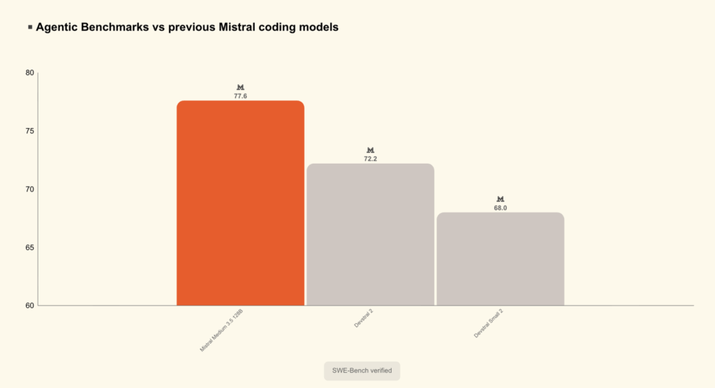
Mistral AI has been quietly building one of the more practical coding agent ecosystems in the open-source/weights AI space, and they are shipping its most significant infrastructure upgrade yet. Mistral team announced remote agents in Vibe, its coding agent platform, alongside the public preview of Mistral Medium 3.5 — a new 128B dense model that now serves as the default model in both Vibe and Le Chat, Mistral’s consumer assistant. What is Vibe, and Why Does It Matter? If you haven’t used it yet, Mistral Vibe is a coding agent accessible through a CLI (command-line interface) that lets an AI model work through software tasks on your behalf — writing code, refactoring modules, generating tests, investigating CI failures, and more. Think of it as a junior developer that never gets tired and can operate across your codebase. Until now, Vibe sessions ran locally, meaning the agent was tied to your laptop and your terminal. That changes today. Remote Agents: The Agent Runs While You Step Away So, basically now coding sessions can work through long tasks while you’re away. Many can run in parallel, and you stop being the bottleneck on every step the agent takes. This is the key behavioral shift. Instead of babysitting a coding session in your terminal, you kick off a task and let the cloud handle the rest. You can start cloud agents from the Mistral Vibe CLI or from Le Chat. While they run, you can inspect what the agent is doing, with file diffs, tool calls, progress states, and questions surfaced as you go. One particularly useful feature for developers already mid-session: ongoing local CLI sessions can be teleported up to the cloud when you want to leave them running, with session history, task state, and approvals carrying across. So you don’t lose your place — you just move the work off your machine. Each session runs in isolation. Each coding session runs in an isolated sandbox, including broad edits and installs. When the work is done, the agent can open a pull request on GitHub and notify you, so you review the result instead of every keystroke that produced it. It’s also worth understanding the logic behind how Vibe connects to Le Chat. Mistral uses Workflows orchestrated in Mistral Studio to bring Mistral Vibe into Le Chat — originally built for their own in-house coding environment, then for enterprise customers, and now open to everyone. This means the remote coding agent in Le Chat is not a standalone feature — it’s built on top of Mistral’s own orchestration layer, which is useful context if you’re thinking about how to architect similar agentic systems yourself. On the integration side, Vibe plugs into GitHub for code and pull requests, Linear and Jira for issues, Sentry for incidents, and apps like Slack or Teams for reporting. Mistral Medium 3.5: The Model Behind It All None of this would be practically possible without a capable underlying AI model. This new released model is Mistral Medium 3.5, which Mistral team describes as its first flagship merged model. It is a dense 128B model with a 256k context window, handling instruction-following, reasoning, and coding in a single set of weights. For context, a 256k context window means the model can process roughly 200,000 words in a single pass — long enough to reason across an entire large codebase. The model is also multimodal. Mistral team trained the vision encoder from scratch to handle variable image sizes and aspect ratios — a notable architectural choice. Most vision-language models reuse pretrained encoders like CLIP, so building this component from scratch suggests Mistral prioritized flexibility in how the model handles real-world image inputs rather than defaulting to fixed-resolution assumptions. Mistral Medium 3.5 scores 77.6% on SWE-Bench Verified, ahead of Devstral 2 and models like Qwen3.5 397B A17B. SWE-Bench Verified is a standard benchmark that tests whether a model can resolve real-world GitHub issues from popular open-source repositories — it’s one of the most reliable proxies for practical software engineering ability. The model also scores 91.4 on τ³-Telecom and has strong agentic capabilities. https://mistral.ai/news/vibe-remote-agents-mistral-medium-3-5 One particularly interesting design choice: reasoning effort is now configurable per request, so the same model can answer a quick chat reply or work through a complex agentic run. This is important for developers integrating the model via API — you can dial down compute for simple lookups and dial it up for multi-step reasoning tasks, without switching models. The model was built for long-horizon tasks, calling multiple tools reliably, and producing structured output that downstream code can consume. Work Mode in Le Chat: A New Agentic Layer Beyond the coding agent upgrades, Mistral is also shipping Work mode in Le Chat — a new agentic mode for more general, multi-step tasks. Work mode is a powerful new agentic mode for complex tasks in Le Chat, powered by a new harness and Mistral Medium 3.5. The agent becomes the execution backend for the assistant itself, so Le Chat can read and write, use several tools at once, and work through multi-step projects until it completes what you’ve asked. Practically, this means things like cross-tool workflows — catching up across email, messages, and calendar; preparing for a meeting with relevant context pulled from multiple sources; or triaging an inbox and creating Jira issues from team discussions. In Work mode, connectors are on by default rather than chosen manually, which lets the agent reach into documents, mailboxes, calendars, and other systems for the rich context it needs to take correct action. This is a significant usability shift from typical chat assistants, where you manually select tools before each session. Transparency is a built-in feature rather than an afterthought: every action the agent takes is visible — you see each tool call and the thinking rationale. Le Chat will ask for explicit approval — based on your permissions — before proceeding with sensitive tasks like sending a message, writing a document, or modifying data. Key Takeaways Here are the key

Mistral AI Launches Remote Agents in Vibe and Mistral Medium 3.5 with 77.6% SWE-Bench Verified Score Read Post »

AI, Committee, 新闻, Uncategorized

What is Tokenization Drift and How to Fix It?

A model can behave perfectly one moment and degrade the next—without any change to your data, pipeline, or logic. The root cause often lies in something far more subtle: how your input is tokenized. Before a model processes text, it converts it into token IDs, and even minor formatting differences—like spacing, line breaks, or punctuation—can produce entirely different token sequences. This phenomenon is known as tokenization drift: when small surface-level changes push your input into a different region of token space, leading to unpredictable shifts in model behavior. The impact goes deeper than just token IDs. During instruction tuning, models learn not only tasks but also the structure in which those tasks are presented—specific separators, prefixes, and formatting patterns. When your prompt deviates from these learned patterns, you are no longer operating within the model’s familiar distribution. The result isn’t confusion—it’s a model doing its best on inputs it was never optimized to handle. In this article, we’ll break this down using the GPT-2 tokenizer to show how small formatting changes affect tokens, and build a simple metric to measure drift across prompts. Then, we’ll implement a lightweight prompt optimization loop to pick formats that keep your inputs consistent and reliable. Setting up the dependencies Copy CodeCopiedUse a different Browser import numpy as np import matplotlib.pyplot as plt import matplotlib.patches as mpatches import seaborn as sns from collections import defaultdict from sklearn.decomposition import PCA In this code block, we are loading the GPT-2 tokenizer — the same Byte-Pair Encoding scheme used by GPT-4, LLaMA, and Mistral. We use GPT-2 specifically because it requires no auth token and demonstrates the space-prefix artifact identically to every modern production tokenizer. Copy CodeCopiedUse a different Browser from transformers import AutoTokenizer tokenizer = AutoTokenizer.from_pretrained(“gpt2”) print(“Tokenizer loaded:”, tokenizer.__class__.__name__) print(“Vocab size:”, tokenizer.vocab_size) Tokenization Artifact Demo We take seven words and test each in two forms—once with a leading space and once without—then encode them using the GPT-2 tokenizer. By setting add_special_tokens=False, we ensure we’re only measuring the token IDs for the words themselves, without any extra padding or special markers. The results are striking. Not a single pair produces the same token ID—every word is treated as completely different depending on whether it has a leading space. Even more interesting, some words without the space don’t map to a single token at all. For example, “classify” becomes two tokens [4871, 1958], while “ classify” is a single token [36509]. This means the model doesn’t just see a different ID—it sees a different sequence length, which shifts how attention is computed for everything that follows. Copy CodeCopiedUse a different Browser pairs = [ (” classify”, “classify”), (” answer”, “answer”), (” positive”, “positive”), (” negative”, “negative”), (” sentiment”, “sentiment”), (” output”, “output”), (” label”, “label”), ] print(“=” * 60) print(f”{‘Token (with space)’:<22} {‘ID’:>6} {‘Token (no space)’:<20} {‘ID’:>6} {‘Same?’:>6}”) print(“=” * 60) for with_space, without_space in pairs: id_ws = tokenizer.encode(with_space, add_special_tokens=False) id_nws = tokenizer.encode(without_space, add_special_tokens=False) match = “✓” if id_ws == id_nws else “✗ DIFFERENT” print(f”{repr(with_space):<22} {str(id_ws):>8} {repr(without_space):<20} {str(id_nws):>8} {match}”) print() print(“Key takeaway: Leading spaces create DIFFERENT token IDs.”) print(“To the model, ‘ classify’ and ‘classify’ are as distinct as ‘apple’ and ‘orange’.”) Visualising the Token ID Shift We plot two charts to make the token ID gap visual. The left chart shows the raw IDs side-by-side — blue for space-prefixed, red for bare — and the right chart plots the absolute distance between each pair. Copy CodeCopiedUse a different Browser words = [p[1] for p in pairs] ids_ws = [tokenizer.encode(” ” + w, add_special_tokens=False)[0] for w in words] ids_nws = [tokenizer.encode(w, add_special_tokens=False)[0] for w in words] delta = [abs(a – b) for a, b in zip(ids_ws, ids_nws)] x = np.arange(len(words)) width = 0.35 fig, axes = plt.subplots(1, 2, figsize=(14, 5)) fig.patch.set_facecolor(“#FAFAF8”) # Left: side-by-side token IDs ax = axes[0] ax.set_facecolor(“#FAFAF8″) bars1 = ax.bar(x – width/2, ids_ws, width, label=’With leading space’, color=”#3B6FE0″, alpha=0.85) bars2 = ax.bar(x + width/2, ids_nws, width, label=’Without leading space’, color=”#E05C3B”, alpha=0.85) ax.set_xticks(x) ax.set_xticklabels(words, rotation=30, ha=”right”, fontsize=9) ax.set_ylabel(“Token ID”, fontsize=10) ax.set_title(“Token IDs: ‘ word’ vs ‘word'”, fontsize=12, fontweight=”bold”, pad=12) ax.legend(fontsize=9) ax.spines[[“top”, “right”]].set_visible(False) ax.grid(axis=”y”, alpha=0.3) for bar in bars1: ax.text(bar.get_x() + bar.get_width()/2, bar.get_height() + 50, str(int(bar.get_height())), ha=”center”, va=”bottom”, fontsize=7, color=”#3B6FE0″) for bar in bars2: ax.text(bar.get_x() + bar.get_width()/2, bar.get_height() + 50, str(int(bar.get_height())), ha=”center”, va=”bottom”, fontsize=7, color=”#E05C3B”) # Right: delta ax2 = axes[1] ax2.set_facecolor(“#FAFAF8”) color_bars = [“#E05C3B” if d > 500 else “#F0A070” if d > 100 else “#A8C4F0” for d in delta] bars3 = ax2.bar(words, delta, color=color_bars, alpha=0.9) ax2.set_ylabel(“Absolute Token ID Distance”, fontsize=10) ax2.set_title(“How Far Apart Are the Token IDs?”, fontsize=12, fontweight=”bold”, pad=12) ax2.set_xticklabels(words, rotation=30, ha=”right”, fontsize=9) ax2.spines[[“top”, “right”]].set_visible(False) ax2.grid(axis=”y”, alpha=0.3) for bar, d in zip(bars3, delta): ax2.text(bar.get_x() + bar.get_width()/2, bar.get_height() + 10, str(d), ha=”center”, va=”bottom”, fontsize=9, fontweight=”bold”) high = mpatches.Patch(color=”#E05C3B”, alpha=0.9, label=”> 500 apart”) med = mpatches.Patch(color=”#F0A070″, alpha=0.9, label=”100-500 apart”) low = mpatches.Patch(color=”#A8C4F0″, alpha=0.9, label=”< 100 apart”) ax2.legend(handles=[high, med, low], fontsize=8) plt.tight_layout(pad=2) plt.suptitle(“Tokenization Artifacts: One Space, Completely Different Token”, fontsize=14, fontweight=”bold”, y=1.02) plt.savefig(“tokenization_artifact.png”, dpi=150, bbox_inches=”tight”, facecolor=”#FAFAF8″) plt.show() Simulating Accuracy Drop Demo We start with a standard SFT prompt format and create a few variations by making small changes—like removing newlines, tweaking punctuation, or rewording the instruction. We then measure how similar each version is using token overlap. The key insight is that even small formatting changes can significantly alter the token sequence. For example, removing newlines drops similarity to around 80%, showing that these aren’t just cosmetic—they’re signals the model relies on. The biggest impact comes from rewording the instruction, which cuts overlap to nearly 50%, meaning the prompt no longer resembles what the model was trained on, increasing the risk of unpredictable behavior. Copy CodeCopiedUse a different Browser def tokenize_prompt(text): return tokenizer.encode(text, add_special_tokens=False) # The canonical SFT (fine-tuning) template — what the model was trained on sft_template = ( “Below is a customer review. Classify the sentiment.nn” “Review: {review}nn” “Sentiment:” ) # Prompt variants — small changes, big token consequences variants = { “✓ SFT template (optimal)”: “Below is a customer review. Classify the sentiment.nnReview: {review}nnSentiment:”, “✗ Removed newlines”: “Below is a customer review. Classify the

What is Tokenization Drift and How to Fix It? Read Post »

AI, Committee, 新闻, Uncategorized

Sakana AI Introduces KAME: A Tandem Speech-to-Speech Architecture That Injects LLM Knowledge in Real Time

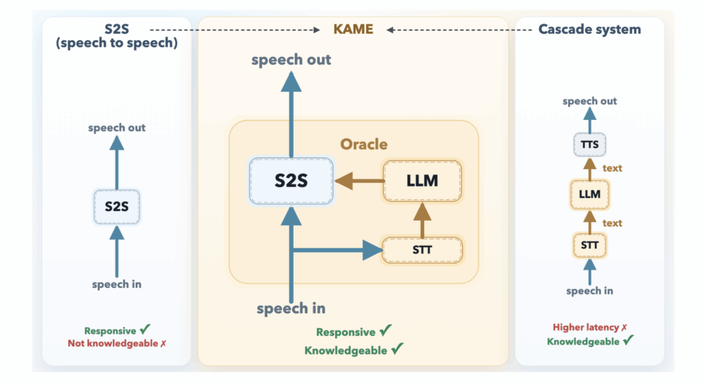
The fundamental tension in conversational AI has always been a binary choice: respond fast or respond smart. Real-time speech-to-speech (S2S) models — the kind that power natural-feeling voice assistants — start talking almost instantly, but their answers tend to be shallow. Cascaded systems that route speech through a large language model (LLM) are far more knowledgeable, but the pipeline delay is long enough to make conversation feel stilted and robotic. Researchers at Sakana AI, the Tokyo-based AI lab introduces KAME (Knowledge-Access Model Extension), a hybrid architecture that keeps the near-zero response latency of a direct S2S system while injecting the richer knowledge of a back-end LLM in real time. The Problem: Two Paradigms, Two Tradeoffs To understand why KAME is important, it helps to understand the two dominant designs it bridges. A direct S2S model like Moshi (developed by KyutAI) is a monolithic transformer that takes in audio tokens and produces audio tokens in a continuous loop. Because it doesn’t need to synchronize with external systems, its response latency is exceptionally low — for many queries, the model starts speaking before the user even finishes their question. But because acoustic signals are far information-denser than text, the model has to spend significant capacity modeling paralinguistic features like tone, emotion, and rhythm. That leaves less room for factual knowledge and deep reasoning. A cascaded system, by contrast, routes the user’s speech through an Automatic Speech Recognition (ASR) model, feeds the resulting text into a powerful LLM, and then converts the LLM’s response back into speech via a Text-to-Speech (TTS) engine. The knowledge quality is excellent — you can plug in any frontier LLM — but the system must wait for the user to finish speaking before ASR and LLM processing can even begin. The result is a median latency of around 2.1 seconds, which is long enough to noticeably interrupt natural conversational flow. https://pub.sakana.ai/kame/ KAME’s Architecture: Speaking While Thinking KAME operates as a tandem system with two asynchronous components running in parallel. The front-end S2S module is based on the Moshi architecture and processes audio in real time at the cycle of discrete audio tokens (approximately every 80 milliseconds). It begins generating a spoken response immediately. Internally, Moshi’s original three-stream design — input audio, inner monologue (text), and output audio — is extended in KAME with a fourth stream: the oracle stream. This is the key innovation point. The back-end LLM module consists of a streaming speech-to-text (STT) component paired with a full-scale LLM. As the user speaks, the STT component continuously builds a partial transcript and periodically sends it to the back-end LLM. For each partial transcript it receives, the LLM generates a candidate text response — called an oracle — and streams it back to the front-end. Because the user’s speech is still arriving, these oracles start as educated guesses and become progressively more accurate as the transcript grows more complete. The front-end S2S transformer then conditions its ongoing speech output on both its own internal context and these incoming oracle tokens. When a new, better oracle arrives, the model can correct course — effectively updating its response mid-sentence, the way a human might. Because both modules run asynchronously and independently, the initial response latency stays near zero. Training on Simulated Oracles One challenge is that no naturally occurring dataset contains oracle signals. Sakana AI research team addresses this with a technique called Simulated Oracle Augmentation. Using a ‘simulator’ LLM and a standard conversational dataset (user utterance + ground-truth response), the research team generates synthetic oracle sequences that mimic what a real-time LLM would produce across different levels of transcript completeness. They define six hint levels (0–5), ranging from a completely unguided guess at hint level 0 to the verbatim ground-truth response at hint level 5. The training data for KAME was built from 56,582 synthetic dialogues drawn from MMLU-Pro, GSM8K, and HSSBench, converted to audio via TTS and augmented with these progressive oracle sequences. Results: Near-Cascaded Quality, Near-Zero Latency Evaluations on a speech-synthesized subset of the MT-Bench multi-turn Q&A benchmark — specifically the reasoning, STEM, and humanities categories (Coding, Extraction, Math, Roleplay, and Writing were excluded as unsuitable for speech interaction) — show a dramatic improvement. Moshi alone scores 2.05 on average. KAME with gpt-4.1 as the back-end scores 6.43, and KAME with claude-opus-4-1 as the back-end scores 6.23 — both at essentially the same latency as Moshi. The leading cascaded system, Unmute (also backed by gpt-4.1), scores 7.70, but with a median latency of 2.1 seconds versus near-zero for KAME. To isolate back-end capability from timing effects, the research team also evaluated the back-end LLM’s text responses from the final oracle injection in each KAME session directly — bypassing the premature-generation problem entirely. Those scores averaged 7.79 (reasoning 6.48, STEM 8.34, humanities 8.56), comparable to Unmute’s 7.70. This confirms that KAME’s gap to cascaded systems is not a ceiling on the back-end LLM’s knowledge, but a consequence of starting to speak before the full user query has been heard. Crucially, KAME is fully back-end agnostic. The front-end was trained using gpt-4.1-nano as the primary back-end, but swapping in claude-opus-4-1 or gemini-2.5-flash at inference time requires no retraining. In Sakana AI’s experiments, claude-opus-4-1 tended to outperform gpt-4.1 on reasoning tasks, while gpt-4.1 scored higher on humanities questions — suggesting practitioners can route queries to the most task-appropriate LLM without touching the front-end model. Key Takeaways KAME bridges the speed-vs-knowledge tradeoff in conversational AI by running a front-end speech-to-speech model and a back-end LLM asynchronously in parallel — the S2S model responds immediately while the LLM continuously injects progressively refined ‘oracle’ signals in real time, shifting the paradigm from ‘think, then speak’ to ‘speak while thinking.’ The performance gains are substantial without any latency cost — KAME raises the MT-Bench score from 2.05 (Moshi baseline) to 6.43, approaching the cascaded system Unmute’s 7.70, while maintaining near-zero median response latency versus Unmute’s 2.1 seconds. The architecture is fully back-end agnostic — the front-end was trained using gpt-4.1-nano but supports

Sakana AI Introduces KAME: A Tandem Speech-to-Speech Architecture That Injects LLM Knowledge in Real Time Read Post »

AI, Committee, 新闻, Uncategorized

Musk v. Altman week 1: Elon Musk says he was duped, warns AI could kill us all, and admits that xAI distills OpenAI’s models

In the first week of the landmark trial between Elon Musk and OpenAI, Musk took the stand in a crisp black suit and tie and argued that OpenAI CEO Sam Altman and president Greg Brockman had deceived him into bankrolling the company. Along the way, he warned that AI could destroy us all and sat through revelations that he had poached OpenAI employees for his own companies. He even confessed, to some audible gasps in the courtroom, that his own AI company, xAI, which makes the chatbot Grok, uses OpenAI’s models to train its own.  The federal courthouse in Oakland, California, was packed with armies of lawyers carrying boxes of exhibits, journalists typing away at their laptops, and a handful of concerned OpenAI employees. Outside, protesters lined the streets, carrying signs urging people to quit ChatGPT, boycott Tesla, or both. Musk looked calm and comfortable, slipping in the occasional quip in his distinct South African accent. But he also was full of remorse.  “I was a fool who provided them free funding to create a startup,” Musk told the jury. He said when he cofounded OpenAI in 2015 with Altman and Brockman, he was donating to a nonprofit developing AI for the benefit of humanity, not to make the executives rich. “I gave them $38 million of essentially free funding, which they then used to create what would become an $800 billion company,” he said. Musk is asking the court to remove Altman and Brockman from their roles and to unwind the restructuring that allowed OpenAI to operate a for-profit subsidiary. The outcome of the trial could upend OpenAI’s race toward an IPO at a valuation approaching $1 trillion. Meanwhile, xAI is expected to go public as a part of Musk’s rocket company SpaceX as early as June, at a target valuation of $1.75 trillion. This week’s testimony revolved around a central question of the trial: why Musk is suing OpenAI. Musk argued he was trying to save OpenAI’s mission to develop AI safely by restoring the company to its original nonprofit structure. OpenAI’s lawyer, William Savitt, who once represented Musk and his electric-car company Tesla, countered that Musk was “never committed to OpenAI being a nonprofit” and instead was suing to undermine his competitor.  Who is the steward of AI safety? During his direct examination early in the week, Musk painted himself as a longtime advocate of AI safety. He said he cofounded OpenAI to create a “counterbalance to Google,” which was leading the AI race at the time. He said that when he asked Google cofounder Larry Page what happens if AI tries to wipe out humanity, Page told him, “That will be fine as long as artificial intelligence survives.”  “The worst-case scenario is a Terminator situation where AI kills us all,” Musk later told the jury. Savitt stood at the lectern and argued that Musk was not a “paladin of safety and regulation.” As he cross-examined Musk in his sharp, surgical cadence, Savitt pointed out that xAI sued the state of Colorado in April over an AI law designed to prevent algorithmic discrimination.  Musk’s lawyer, Steven Molo, sprang to his feet to object. He asked the judge if he, too, could weigh in on ChatGPT’s safety record.  The lawyers then entered a heated debate about who was the true guardian of AI safety.  The sparring continued the next morning. “We all could die as a result of artificial intelligence!” said Molo, suggesting that OpenAI could not be trusted to build AI safely. “Despite these risks, your client is creating a company that’s in the exact space,” Judge Yvonne Gonzalez Rogers said sternly, referring to xAI. “I suspect there’s plenty of people who don’t want to put the future of humanity in Mr. Musk’s hands.” When the lawyers began talking over each other, the judge snapped. “This is not a trial on whether or not artificial intelligence has damaged humanity,” she said.  When did Musk think he was being duped? As Savitt continued to cross-examine Musk, he pressed on the idea that Musk had never been committed to keeping OpenAI a nonprofit. He also claimed that Musk waited too long to sue OpenAI, filing after the statute of limitations ran out.  Musk explained why he sued in 2024 rather than earlier, describing “three phases” in his views of OpenAI. In phase one, he was “enthusiastically supportive” of the company.” In phase two, “I started to lose confidence that they were telling me the truth,” he said. In phase three, “I’m sure they’re looting the nonprofit.”  In 2017, Musk and other OpenAI cofounders discussed creating a for-profit subsidiary to raise enough capital to build artificial general intelligence—powerful AI that can compete with humans on most cognitive tasks. Musk wanted a majority interest in the subsidiary and the right to choose a majority of the board members. He also pitched having Tesla acquire OpenAI. (He left OpenAI in 2018.) “I was not opposed to there being a small for-profit that provides funding to the nonprofit,” he told the jury, “as long as the tail didn’t wag the dog.”  But it was only in late 2022, Musk testified, that he “lost trust in Altman” and his commitment to keeping the company a nonprofit. The key moment came, he said, when he learned that Microsoft would invest $10 billion in OpenAI.  “I texted Sam Altman, ‘What the hell is going on? This is a bait and switch,’” he told the jury. Microsoft would give $10 billion only if it expected “a very big financial return,” he said. Is Musk just trying to kill competition? But Savitt argued that Musk was really suing to undermine OpenAI as a competitor to his empire of tech companies. While he was on the board of OpenAI, Musk was also running Tesla and his brain-implant company, Neuralink. He founded xAI in 2023. Savitt pulled up an email that Musk had sent to a Tesla vice president in 2017 after hiring Andrej Karpathy, a founding member of OpenAI,

Musk v. Altman week 1: Elon Musk says he was duped, warns AI could kill us all, and admits that xAI distills OpenAI’s models Read Post »

AI, Committee, 新闻, Uncategorized

A Coding Implementation of End-to-End Brain Decoding from MEG Signals Using NeuralSet and Deep Learning for Predicting Linguistic Features

In this tutorial, we explore how we can decode linguistic features directly from brain signals using a modern neuroAI pipeline. We work with MEG data and build an end-to-end system that transforms raw neural activity into meaningful predictions, in this case, estimating word length from brain responses. We set up the environment, load and process neural events, design a custom feature extractor, and construct a structured data pipeline using NeuralSet. From there, we train a convolutional neural network to learn patterns in the temporal and spatial structure of MEG signals. Throughout the process, we focus on building a clean, modular workflow that mirrors real-world neuroAI research practices. Copy CodeCopiedUse a different Browser import subprocess, sys, importlib, pkgutil def pip_install(*pkgs): print(f”pip install {‘ ‘.join(pkgs)} …”) r = subprocess.run([sys.executable, “-m”, “pip”, “install”, “-q”, *pkgs], capture_output=True, text=True) if r.returncode != 0: print(“pip STDOUT:”, r.stdout[-2000:]) print(“pip STDERR:”, r.stderr[-2000:]) raise RuntimeError(“pip install failed; see output above.”) print(” ok”) pip_install(“numpy>=2.0,<2.3”) pip_install(“neuralset”) pip_install(“neuralfetch”) import numpy as np from numpy._core.umath import _center print(f”numpy {np.__version__} OK”) import warnings, typing as tp warnings.filterwarnings(“ignore”) import pandas as pd import torch import torch.nn as nn import torch.nn.functional as F from torch.utils.data import DataLoader import matplotlib.pyplot as plt import neuralset as ns from neuralset import extractors as ext_mod We install and validate all required dependencies, ensuring critical packages such as NumPy and NeuralSet are properly configured. We perform a quick NumPy check to avoid runtime issues later in the pipeline. We then import all core libraries needed for data processing, modeling, and visualization. Copy CodeCopiedUse a different Browser def deep_import(pkg_name: str): try: pkg = importlib.import_module(pkg_name) except Exception as e: print(f” could not import {pkg_name}: {e}”) return if not hasattr(pkg, “__path__”): return for m in pkgutil.walk_packages(pkg.__path__, prefix=pkg_name + “.”): try: importlib.import_module(m.name) except Exception: pass deep_import(“neuralfetch”) deep_import(“neuralset”) torch.manual_seed(0); np.random.seed(0) catalog = ns.Study.catalog() print(f”n{len(catalog)} studies registered.”) preferred = [“Fake2025Meg”, “Test2025Meg”, “Test2023Meg”] study_name = next((n for n in preferred if n in catalog), None) if study_name is None: meg_studies = [n for n, c in catalog.items() if “Meg” in c.neuro_types()] study_name = meg_studies[0] if meg_studies else None if study_name is None: raise RuntimeError( “No MEG study available. Catalog: ” f”{sorted(catalog.keys())[:20]}… ” “Install neuralfetch correctly (pip install neuralfetch) and re-run.” ) print(f”→ Using study: {study_name}”) We dynamically import all submodules from NeuralFetch and NeuralSet to ensure that all available studies are properly registered. We seed the random number generator for reproducibility and inspect the study catalog to identify available MEG datasets. We then select an appropriate study to use as the foundation for our pipeline. Copy CodeCopiedUse a different Browser class CharCount(ext_mod.BaseStatic): event_types: tp.Literal[“Word”] = “Word” def get_static(self, event) -> torch.Tensor: return torch.tensor([float(len(event.text))], dtype=torch.float32) print(“nBuilding chain…”) chain = ns.Chain(steps=[ {“name”: study_name, “path”: str(ns.CACHE_FOLDER)}, {“name”: “QueryEvents”, “query”: “type in [‘Word’, ‘Meg’]”}, ]) events = chain.run() print(f” → {len(events)} events; types={sorted(events.type.unique().tolist())}”) print(f” → Words: {(events.type==’Word’).sum()} | ” f”timelines: {events.timeline.nunique()}”) print(“nSample words:”) print(events[events.type==’Word’][[“start”,”duration”,”text”,”timeline”]] .head(5).to_string(index=False)) print(“nBuilding segmenter…”) segmenter = ns.dataloader.Segmenter( extractors={ “meg”: {“name”: “MegExtractor”, “frequency”: 100.0}, “char_count”: CharCount(aggregation=”trigger”), }, trigger_query=”type == ‘Word'”, start=-0.2, duration=0.8, drop_incomplete=True, ) dataset = segmenter.apply(events) print(f” → SegmentDataset: {len(dataset)} segments”) s0 = dataset[0] print(f”nSingle item:n meg : {tuple(s0.data[‘meg’].shape)}”) print(f” char_count : {s0.data[‘char_count’].item()} ” f”(word: {s0.segments[0].trigger.text!r})”) We define a custom extractor that computes the character count of each word event, enabling us to create a supervised learning target. We build a processing chain to load and filter relevant events from the selected study. We then segment the MEG signals around word events and construct a dataset ready for modeling. Copy CodeCopiedUse a different Browser rng = np.random.RandomState(42) perm = rng.permutation(len(dataset)) n_tr, n_va = int(0.70*len(dataset)), int(0.15*len(dataset)) train_ds = dataset.select(perm[:n_tr]) val_ds = dataset.select(perm[n_tr:n_tr+n_va]) test_ds = dataset.select(perm[n_tr+n_va:]) print(f”nSplit | train={len(train_ds)} val={len(val_ds)} test={len(test_ds)}”) mk = lambda d, sh: DataLoader(d, batch_size=32, shuffle=sh, collate_fn=d.collate_fn, drop_last=False) train_loader, val_loader, test_loader = mk(train_ds, True), mk(val_ds, False), mk(test_ds, False) probe = next(iter(train_loader)) n_ch, n_t = probe.data[“meg”].shape[-2:] print(f” → batch[meg] shape: {tuple(probe.data[‘meg’].shape)}”) print(f” → batch[char] shape: {tuple(probe.data[‘char_count’].shape)}”) class MEGDecoder(nn.Module): def __init__(self, n_channels: int, mid: int = 64): super().__init__() self.spatial = nn.Conv1d(n_channels, mid, 1) self.bn0 = nn.BatchNorm1d(mid) self.temporal1 = nn.Conv1d(mid, mid, 7, padding=3) self.bn1 = nn.BatchNorm1d(mid) self.temporal2 = nn.Conv1d(mid, mid//2, 7, padding=3) self.bn2 = nn.BatchNorm1d(mid//2) self.pool = nn.AdaptiveAvgPool1d(1) self.head = nn.Linear(mid//2, 1) self.drop = nn.Dropout(0.3) def forward(self, x): x = F.gelu(self.bn0(self.spatial(x))) x = F.gelu(self.bn1(self.temporal1(x))) x = self.drop(x) x = F.gelu(self.bn2(self.temporal2(x))) return self.head(self.pool(x).squeeze(-1)).squeeze(-1) device = torch.device(“cuda” if torch.cuda.is_available() else “cpu”) model = MEGDecoder(n_channels=n_ch).to(device) print(f”nDevice: {device} | params: {sum(p.numel() for p in model.parameters()):,}”) train_targets = torch.cat([b.data[“char_count”].squeeze(-1) for b in train_loader]) y_mean, y_std = train_targets.mean().item(), train_targets.std().item() + 1e-6 print(f”Target μ={y_mean:.2f} σ={y_std:.2f}”) def prep(batch): x = batch.data[“meg”].to(device).float() y = batch.data[“char_count”].squeeze(-1).to(device).float() x = (x – x.mean(-1, keepdim=True)) / (x.std(-1, keepdim=True) + 1e-6) y = (y – y_mean) / y_std return x, y We split the dataset into training, validation, and test sets to ensure proper model evaluation. We create data loaders and inspect batch shapes to confirm correct data formatting. We then define a convolutional neural network and prepare normalized inputs and targets for stable training. Copy CodeCopiedUse a different Browser EPOCHS = 15 opt = torch.optim.AdamW(model.parameters(), lr=1e-3, weight_decay=1e-4) sched = torch.optim.lr_scheduler.CosineAnnealingLR(opt, T_max=EPOCHS) loss_fn = nn.MSELoss() hist = {“tr”: [], “va”: [], “r”: []} def pearson(a, b): a, b = a – a.mean(), b – b.mean() return (a*b).sum() / (a.norm()*b.norm() + 1e-8) print(“n” + “=”*64) print(f”{‘Epoch’:>5} | {‘train’:>9} | {‘val’:>9} | {‘val_r’:>7}”) print(“=”*64) for ep in range(EPOCHS): model.train(); tr = [] for batch in train_loader: x, y = prep(batch) loss = loss_fn(model(x), y) opt.zero_grad(); loss.backward() torch.nn.utils.clip_grad_norm_(model.parameters(), 1.0) opt.step(); tr.append(loss.item()) sched.step() model.eval(); va, P, T = [], [], [] with torch.no_grad(): for batch in val_loader: x, y = prep(batch); p = model(x) va.append(loss_fn(p, y).item()); P.append(p.cpu()); T.append(y.cpu()) P, T = torch.cat(P), torch.cat(T) r = pearson(P, T).item() hist[“tr”].append(np.mean(tr)); hist[“va”].append(np.mean(va)); hist[“r”].append(r) print(f”{ep+1:>5d} | {np.mean(tr):>9.4f} | {np.mean(va):>9.4f} | {r:>+7.3f}”) model.eval(); P, T = [], [] with torch.no_grad(): for batch in test_loader: x, y = prep(batch) P.append(model(x).cpu()); T.append(y.cpu()) P, T = torch.cat(P), torch.cat(T) test_r = pearson(P, T).item() test_mse = ((P – T) ** 2).mean().item() print(f”nTEST | Pearson r = {test_r:+.3f} MSE = {test_mse:.3f}”) print(f”(Synthetic-MEG signals are random by design — small/zero r is expected.)”) fig, ax = plt.subplots(1, 3, figsize=(15, 4))

A Coding Implementation of End-to-End Brain Decoding from MEG Signals Using NeuralSet and Deep Learning for Predicting Linguistic Features Read Post »

AI, Committee, 新闻, Uncategorized

Meta Introduces Autodata: An Agentic Framework That Turns AI Models into Autonomous Data Scientists for High-Quality Training Data Creation

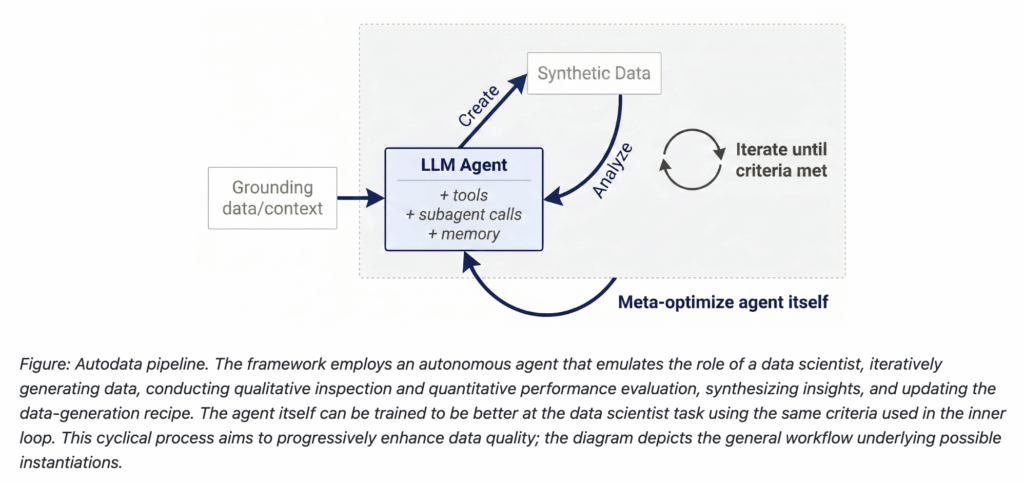
The bottleneck in building better AI models has never been compute alone — it has always been data quality. Meta AI’s RAM (Reasoning, Alignment, and Memory) team is now addressing that bottleneck directly. Meta researchers have introduced Autodata, a framework that deploys AI agents in the role of an autonomous data scientist, tasked with iteratively building, evaluating, and refining training and evaluation datasets — without relying on costly human annotation at every step. And the results, tested on complex scientific reasoning problems, show that this approach doesn’t just match classical synthetic data generation methods — it significantly outperforms them. https://facebookresearch.github.io/RAM/blogs/autodata/ Why Synthetic Data Creation Has Always Been Hard To understand what Autodata is solving, you need to understand how AI training data is typically created today. Most modern AI systems started with human-written data. As models improved, researchers began supplementing that with synthetic data — data generated by the model itself. Synthetic data is attractive because it can generate rare edge cases, reduce the cost of manual labeling, and produce more challenging examples than what naturally exists in public corpora. The dominant approach for generating synthetic data has been Self-Instruct — prompting a large language model (LLM) using zero-shot or few-shot examples to create new training samples. Grounded Self-Instruct methods extended that by grounding generation on documents and other sources to reduce hallucination and increase diversity. CoT Self-Instruct (Chain-of-Thought Self-Instruct) pushed further by using chain-of-thought reasoning during generation to construct more complex tasks more accurately. Most recently, “Self-Challenging” methods allow a challenger agent to interact with tools before proposing a task and accompanying evaluation functions — the closest prior work to what Autodata does. The problem? None of these methods gave researchers a feedback-driven way to actually control or iteratively improve data quality during generation itself. You could filter, evolve, or refine data after the fact — but the generation pipeline remained largely static and single-pass. Autodata changes that. https://facebookresearch.github.io/RAM/blogs/autodata/ What Autodata Actually Does Autodata is a method that allows AI agents to act as data scientists who iteratively build high-quality training and evaluation data. Instead of generating data in a single pass, the agent runs a closed-loop pipeline modeled after how a human data scientist actually works: Data Creation — The agent grounds itself on provided source documents (research papers, code, legal text, etc.) and uses tools and learned skills to generate training or evaluation examples. Data Analysis — The agent then inspects what it created: Is this example correct? High quality? Challenging enough? It synthesizes learnings at the example level and, eventually, at the dataset level (Is it diverse? Does it improve a model when used as training data?). Iteration — Using those learnings, the agent updates its data-generation recipe and loops back to create better data. This continues until a stopping criterion is met. Agentic data creation provides a way to convert increased inference compute into higher quality model training. The more inference-time compute you give the agent, the better the data it produces — a key insight for practitioners managing compute budgets. The Specific Implementation: Agentic Self-Instruct Meta’s initial instantiation of Autodata is called Agentic Self-Instruct, and its architecture is built around a main orchestrator LLM that coordinates four specialized subagents: Challenger LLM — generates a training example (input + response pair) based on a detailed prompt from the main agent Weak Solver — a smaller, less capable model expected to generally fail on the generated example Strong Solver — a more capable model expected to generally succeed Verifier/Judge — evaluates whether each solver’s output meets quality criteria, using rubrics generated by the Challenger LLM An important design note: the Weak and Strong solver can actually be the same LLM operating in different modes. For example, the strong version can be allowed to use increased inference time compute including scaffolding or aggregation, as well as having access to privileged information — giving practitioners flexibility in how they define capability separation. The acceptance criteria are precise and multi-condition. For an example to be accepted into the dataset, all four of the following must hold: The quality verifier (QV) must pass the example weak_avg ≤ 65% and max_weak ≤ 75% with no zero scores strong_avg ≥ 60% and strong_avg < 95% — ensuring the question is neither too hard for everyone nor trivially easy for the strong solver The gap strong_avg − weak_avg ≥ 20% If any of those thresholds aren’t met, the main agent sends targeted feedback to the Challenger and tries again — from a different reasoning angle. This loop typically runs several rounds per paper (median 3–5) before producing an accepted question or exhausting its step budget. The Numbers That Matter The quality gains over standard CoT Self-Instruct are measurable and significant. Under CoT Self-Instruct, the two solvers score nearly identically — weak at 71.4% and strong at 73.3%, a gap of only 1.9 percentage points — showing that single-shot questions fail to find challenging enough tasks for either model. Agentic Self-Instruct drives the weak score down to 43.7% while lifting the strong score to 77.8%, widening the gap to 34 points. The agentic data creation loop produces questions that specifically reward stronger model capabilities, rather than questions both models can answer equally well. The dataset itself was produced by processing over 10,000 CS papers from the S2ORC corpus (2022+), yielding 2,117 QA pairs that satisfy all quality constraints and performance gap requirements. When Qwen-3.5-4B was then trained with GRPO for roughly one epoch (batch size 32, learning rate 1e-6) on Agentic Self-Instruct data versus CoT Self-Instruct data — using Kimi-K2.6 as the reward model to score responses against the generated rubrics — the model trained on agentic data demonstrated a clear advantage on both in-distribution and out-of-distribution test sets. Meta-Optimization: Teaching the Agent to Be a Better Data Scientist Autodata goes one level deeper. Beyond the inner data creation loop, the framework supports meta-optimization of the data scientist agent itself — using the same inner-loop quality criteria to optimize the outer-loop agent harness

Meta Introduces Autodata: An Agentic Framework That Turns AI Models into Autonomous Data Scientists for High-Quality Training Data Creation Read Post »

AI, Committee, 新闻, Uncategorized

A New NVIDIA Research Shows Speculative Decoding in NeMo RL Achieves 1.8× Rollout Generation Speedup at 8B and Projects 2.5× End-to-End Speedup at 235B

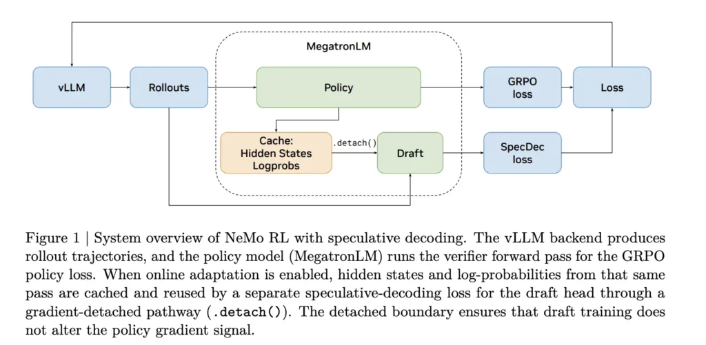
If you have been running reinforcement learning (RL) post-training on a language model for math reasoning, code generation, or any verifiable task, you have almost certainly stared at a progress bar while your GPU cluster burns through rollout generation. A team of researchers from NVIDIA proposes a precise fix by integrating speculative decoding into the RL training loop itself, and do it in a way that preserves the target model’s exact output distribution. The research team integrated speculative decoding directly into NeMo RL v0.6.0 with a vLLM backend, delivering lossless rollout acceleration at both 8B and projected 235B model scales.The latest NeMo RL v0.6.0 release officially ships speculative decoding as a supported feature alongside the SGLang backend, the Muon optimizer, and YaRN long-context training. https://arxiv.org/pdf/2604.26779 Why Rollout Generation is the Bottleneck To understand the problem, it helps to know how a synchronous RL training step breaks down. In NeMo RL, each step consists of five stages: data loading, weight synchronization and backend preparation (prepare), rollout generation (gen), log-probability recomputation (logprob), and policy optimization (train). The research team measured this breakdown on Qwen3-8B under two workloads — RL-Think, which continues training a reasoning-capable model, and RL-Zero, which starts from a base model and learns reasoning from scratch. In both cases, rollout generation accounts for 65–72% of total step time. Log-probability recomputation and training together take only about 27–33%. This makes generation the only stage worth targeting for acceleration, and the one that determines the ceiling for any rollout-side optimization. https://arxiv.org/pdf/2604.26779 What Speculative Decoding Actually Does Speculative decoding is a technique where a smaller, faster draft model proposes several tokens at once, and the larger target model (the one you are actually training) verifies them using a rejection sampling procedure. The key property and why it matters for RL, is that the rejection procedure is mathematically guaranteed to produce the same output distribution as if the target model had generated those tokens autoregressively. No distribution mismatch, no off-policy corrections needed, no change to the training signal. This is important because in RL post-training, the training reward depends on the policy’s own samples. Methods like asynchronous execution, off-policy replay, or low-precision rollouts all trade some amount of training fidelity for throughput. Speculative decoding trades nothing: the rollouts are identical in distribution to what the target model would have generated on its own, just produced faster. The System Integration Challenge Adding a draft model to a serving backend is straightforward. Adding one to an RL training loop is not. Every time the policy updates, the rollout engine must receive new weights. The draft model must remain aligned with the evolving policy. Log-probabilities, KL penalties, and the GRPO policy loss must all be computed against the target (verifier) policy not the draft or the optimization target is silently corrupted. The NVIDIA research team handles this in NeMo RL with a two-path architecture. The general path uses EAGLE-3, a drafting framework that works with any pretrained model without requiring native multi-token prediction (MTP) support. A native path is also available for models that ship with built-in MTP heads. When online draft adaptation is enabled, the hidden states and log-probabilities from the MegatronLM verifier forward pass are cached and reused to supervise the draft head via a gradient-detached pathway, so draft training never interferes with the policy gradient signal. Measured Results at 8B Scale On 32 GB200 GPUs (8 GB200 NVL72 nodes, 4 GPUs per node), EAGLE-3 reduces generation latency from 100 seconds to 56.6 seconds on RL-Zero — a 1.8× generation speedup. On RL-Think, it drops from 133.6 seconds to 87.0 seconds, a 1.54× speedup. Because log-probability re-computation and training are unchanged, these generation-side gains translate to overall step speedups of 1.41× on RL-Zero and 1.35× on RL-Think. Validation accuracy on AIME-2024 evolves identically under autoregressive and speculative decoding throughout training, confirming that the lossless guarantee holds in practice. The research team also tests n-gram drafting as a model-free speculative baseline. Despite achieving acceptance lengths of 2.47 on RL-Zero and 2.05 on RL-Think, n-gram drafting is slower than the autoregressive baseline in both settings — 0.7× and 0.5× respectively. This is a critical finding for practitioners: a positive acceptance length is necessary but not sufficient. If the verification overhead is high enough, speculation makes things worse. Three Configuration Decisions That Determine Realized Speedup The research team isolates three operational choices that practitioners must get right. Draft initialization matters more than generic drafting ability. An EAGLE-3 draft initialized on the DAPO post-training dataset achieves a 1.77× generation speedup on RL-Zero, while a draft initialized on the general-purpose UltraChat and Magpie datasets achieves only 1.51× at the same draft length. The draft must be aligned with the actual rollout distribution encountered during RL, not just a broad chat distribution. Draft length has a non-obvious optimum. At draft length k=3, RL-Zero achieves 1.77× speedup and RL-Think achieves 1.53×. Increasing to k=5 raises the acceptance length but drops speedup to 1.44× on RL-Zero and 0.84× on RL-Think — the latter already slower than autoregressive. At k=7, RL-Zero drops further to 1.21× and RL-Think to 0.71×. The contrast matters: RL-Zero’s rollouts are generated from a base model starting with short outputs, making them easier for the draft to predict even at high k. RL-Think’s fully developed reasoning traces are harder to speculate over, so the overhead of longer drafts erases the benefit sooner. More speculative work per step can erase the benefit of higher acceptance entirely, especially in harder generation regimes. Online draft adaptation — updating the draft during RL using rollouts generated by the current policy helps most when the draft is weakly initialized. For a DAPO-initialized draft, offline and online configurations perform nearly identically (1.77× vs. 1.78× on RL-Zero). For a UltraChat-initialized draft, online updating improves speedup from 1.51× to 1.63× on RL-Zero. Interaction with asynchronous execution was also tested directly at 8B scale not just in simulation. The research team ran RL-Think at policy lag 1 in a 16-node non-colocated configuration, with 12 nodes dedicated to generation

A New NVIDIA Research Shows Speculative Decoding in NeMo RL Achieves 1.8× Rollout Generation Speedup at 8B and Projects 2.5× End-to-End Speedup at 235B Read Post »

AI, Committee, 新闻, Uncategorized

A Coding Implementation to Parsing, Analyzing, Visualizing, and Fine-Tuning Agent Reasoning Traces Using the lambda/hermes-agent-reasoning-traces Dataset

In this tutorial, we explore the lambda/hermes-agent-reasoning-traces dataset to understand how agent-based models think, use tools, and generate responses across multi-turn conversations. We start by loading and inspecting the dataset, examining its structure, categories, and conversational format to get a clear idea of the available information. We then build simple parsers to extract key components such as reasoning traces, tool calls, and tool responses, allowing us to separate internal thinking from external actions. Also, we analyze patterns such as tool usage frequency, conversation length, and error rates to better understand agent behavior. We also create visualizations to highlight these trends and make the analysis more intuitive. Finally, we prepare the dataset for training by converting it into a model-friendly format, making it suitable for tasks like supervised fine-tuning. Copy CodeCopiedUse a different Browser !pip -q install -U datasets pandas matplotlib seaborn transformers accelerate trl import json, re, random, textwrap from collections import Counter, defaultdict import pandas as pd import numpy as np import matplotlib.pyplot as plt from datasets import load_dataset, concatenate_datasets random.seed(0) CONFIG = “kimi” ds = load_dataset(“lambda/hermes-agent-reasoning-traces”, CONFIG, split=”train”) print(ds) print(“Config:”, CONFIG, “| Fields:”, ds.column_names) print(“Categories:”, sorted(set(ds[“category”]))) COMPARE_BOTH = False if COMPARE_BOTH: ds_kimi = load_dataset(“lambda/hermes-agent-reasoning-traces”, “kimi”, split=”train”) ds_glm = load_dataset(“lambda/hermes-agent-reasoning-traces”, “glm-5.1″, split=”train”) ds_kimi = ds_kimi.add_column(“source”, [“kimi”] * len(ds_kimi)) ds_glm = ds_glm.add_column(“source”, [“glm-5.1”] * len(ds_glm)) ds = concatenate_datasets([ds_kimi, ds_glm]).shuffle(seed=0) print(“Combined:”, ds, “→ counts:”, Counter(ds[“source”])) sample = ds[0] print(“n=== Sample 0 ===”) print(“id :”, sample[“id”]) print(“category :”, sample[“category”], “/”, sample[“subcategory”]) print(“task :”, sample[“task”]) print(“turns :”, len(sample[“conversations”])) print(“system[0] :”, sample[“conversations”][0][“value”][:220], “…n”) We install all required libraries and import the necessary modules to set up our environment. We then load the lambda/hermes-agent-reasoning-traces dataset and inspect its structure, fields, and categories. We also optionally combine multiple dataset configurations and examine a sample to understand the conversational format. Copy CodeCopiedUse a different Browser THINK_RE = re.compile(r”<think>(.*?)</think>”, re.DOTALL) TOOL_CALL_RE = re.compile(r”<tool_call>s*({.*?})s*</tool_call>”, re.DOTALL) TOOL_RESP_RE = re.compile(r”<tool_response>s*(.*?)s*</tool_response>”, re.DOTALL) def parse_assistant(value: str) -> dict: thoughts = [t.strip() for t in THINK_RE.findall(value)] calls = [] for raw in TOOL_CALL_RE.findall(value): try: calls.append(json.loads(raw)) except json.JSONDecodeError: calls.append({“name”: “<malformed>”, “arguments”: {}}) final = TOOL_CALL_RE.sub(“”, THINK_RE.sub(“”, value)).strip() return {“thoughts”: thoughts, “tool_calls”: calls, “final”: final} def parse_tool(value: str): raw = TOOL_RESP_RE.search(value) if not raw: return {“raw”: value} body = raw.group(1) try: return json.loads(body) except: return {“raw”: body} first_gpt = next(t for t in sample[“conversations”] if t[“from”] == “gpt”) p = parse_assistant(first_gpt[“value”]) print(“Thought preview :”, (p[“thoughts”][0][:160] + “…”) if p[“thoughts”] else “(none)”) print(“Tool calls :”, [(c.get(“name”), list(c.get(“arguments”, {}).keys())) for c in p[“tool_calls”]]) We define regex-based parsers to extract reasoning traces, tool calls, and tool responses from the dataset. We process assistant messages to separate thoughts, actions, and final outputs in a structured way. We then test the parser on a sample conversation to verify that the extraction works correctly. Copy CodeCopiedUse a different Browser N = 3000 sub = ds.select(range(min(N, len(ds)))) tool_calls = Counter() parallel_widths = Counter() thoughts_per_turn = [] calls_per_traj = [] errors_per_traj = [] turns_per_traj = [] cat_counts = Counter() for ex in sub: cat_counts[ex[“category”]] += 1 n_calls = n_err = 0 turns_per_traj.append(len(ex[“conversations”])) for t in ex[“conversations”]: if t[“from”] == “gpt”: p = parse_assistant(t[“value”]) thoughts_per_turn.append(len(p[“thoughts”])) if p[“tool_calls”]: parallel_widths[len(p[“tool_calls”])] += 1 for c in p[“tool_calls”]: tool_calls[c.get(“name”, “<unknown>”)] += 1 n_calls += len(p[“tool_calls”]) elif t[“from”] == “tool”: r = parse_tool(t[“value”]) blob = json.dumps(r).lower() if “error” in blob or ‘”exit_code”: 1’ in blob or “traceback” in blob: n_err += 1 calls_per_traj.append(n_calls) errors_per_traj.append(n_err) print(f”nScanned {len(sub)} trajectories”) print(f”Avg turns/traj : {np.mean(turns_per_traj):.1f}”) print(f”Avg tool calls/traj : {np.mean(calls_per_traj):.1f}”) print(f”% with >=1 error : {100*np.mean([e>0 for e in errors_per_traj]):.1f}%”) print(f”% parallel turns : {100*sum(v for k,v in parallel_widths.items() if k>1)/max(1,sum(parallel_widths.values())):.1f}%”) print(“Top 10 tools :”, tool_calls.most_common(10)) fig, axes = plt.subplots(2, 2, figsize=(13, 9)) top = tool_calls.most_common(15) axes[0,0].barh([t for t,_ in top][::-1], [c for _,c in top][::-1], color=”teal”) axes[0,0].set_title(“Top 15 tools by call volume”) axes[0,0].set_xlabel(“calls”) ks = sorted(parallel_widths) axes[0,1].bar([str(k) for k in ks], [parallel_widths[k] for k in ks], color=”coral”) axes[0,1].set_title(“Tool-calls per assistant turn (parallel width)”) axes[0,1].set_xlabel(“# tool calls in one turn”); axes[0,1].set_ylabel(“count”) axes[0,1].set_yscale(“log”) axes[1,0].hist(turns_per_traj, bins=40, color=”steelblue”) axes[1,0].set_title(“Conversation length”); axes[1,0].set_xlabel(“turns”) cats, vals = zip(*cat_counts.most_common()) axes[1,1].pie(vals, labels=cats, autopct=”%1.0f%%”, startangle=90) axes[1,1].set_title(“Category distribution”) plt.tight_layout(); plt.show() We perform dataset-wide analytics to measure tool usage, conversation lengths, and error patterns. We aggregate statistics across multiple samples to understand overall agent behavior. We also create visualizations to highlight trends such as tool frequency, parallel calls, and category distribution. Copy CodeCopiedUse a different Browser def render_trace(ex, max_chars=350): print(f”n{‘=’*72}nTASK [{ex[‘category’]} / {ex[‘subcategory’]}]: {ex[‘task’]}n{‘=’*72}”) for t in ex[“conversations”]: role = t[“from”] if role == “system”: continue if role == “human”: print(f”n[USER]n{textwrap.shorten(t[‘value’], 600)}”) elif role == “gpt”: p = parse_assistant(t[“value”]) for th in p[“thoughts”]: print(f”n[THINK]n{textwrap.shorten(th, max_chars)}”) for c in p[“tool_calls”]: args = json.dumps(c.get(“arguments”, {}))[:200] print(f”[CALL] {c.get(‘name’)}({args})”) if p[“final”]: print(f”n[ANSWER]n{textwrap.shorten(p[‘final’], max_chars)}”) elif role == “tool”: print(f”[TOOL_RESPONSE] {textwrap.shorten(t[‘value’], 220)}”) print(“=”*72) idx = int(np.argmin(np.abs(np.array(turns_per_traj) – 10))) render_trace(sub[idx]) def get_tool_schemas(ex): try: return json.loads(ex[“tools”]) except: return [] schemas = get_tool_schemas(sample) print(f”nSample 0 has {len(schemas)} tools available”) for s in schemas[:3]: fn = s.get(“function”, {}) print(” -“, fn.get(“name”), “—”, (fn.get(“description”) or “”)[:80]) ROLE_MAP = {“system”: “system”, “human”: “user”, “gpt”: “assistant”, “tool”: “tool”} def to_openai_messages(conv): return [{“role”: ROLE_MAP[t[“from”]], “content”: t[“value”]} for t in conv] example_msgs = to_openai_messages(sample[“conversations”]) print(“nFirst 2 OpenAI messages:”) for m in example_msgs[:2]: print(” “, m[“role”], “→”, m[“content”][:120].replace(“n”, ” “), “…”) We build utilities to render full conversation traces in a readable format for deeper inspection. We also extract tool schemas and convert the dataset into OpenAI-style message format for compatibility with training pipelines. This helps us better understand both the structure of tools and how conversations can be standardized. Copy CodeCopiedUse a different Browser from transformers import AutoTokenizer TOK_ID = “Qwen/Qwen2.5-0.5B-Instruct” tok = AutoTokenizer.from_pretrained(TOK_ID) def build_masked(conv, tokenizer, max_len=2048): msgs = to_openai_messages(conv) for m in msgs: if m[“role”] == “tool”: m[“role”] = “user” m[“content”] = “[TOOL OUTPUT]n” + m[“content”] input_ids, labels = [], [] for m in msgs: text = tokenizer.apply_chat_template([m], tokenize=False, add_generation_prompt=False) ids = tokenizer.encode(text, add_special_tokens=False) input_ids.extend(ids) labels.extend(ids if m[“role”] == “assistant” else [-100] * len(ids)) return input_ids[:max_len], labels[:max_len] ids, lbls = build_masked(sample[“conversations”], tok) trainable = sum(1 for x in lbls if x != -100) print(f”nTokenized example: {len(ids)} tokens, {trainable} trainable ({100*trainable/len(ids):.1f}%)”) think_lens, call_lens, ans_lens = [], [], []

A Coding Implementation to Parsing, Analyzing, Visualizing, and Fine-Tuning Agent Reasoning Traces Using the lambda/hermes-agent-reasoning-traces Dataset Read Post »

AI, Committee, 新闻, Uncategorized

Trump’s mass firing just dealt another blow to American science

This past week delivered another gut punch for science in the US. This time, the target was the National Science Foundation—a federal agency that funds major research projects to the tune of around $9 billion. The foundation’s efforts were overseen by a board of 22 prominent scientists. On Friday last week, they were all fired. The NSF has been without a director since April 2025, when former director Sethuraman Panchanathan stepped down in the wake of DOGE-led funding cuts and mass firings. Trump’s nominee for the role is Jim O’Neill, an investor and longevity enthusiast who does not have a science background. It’s hard to predict exactly how things will shake out for science. But it’s not looking great. The NSF was established in 1950 to “promote the progress of science,” among other goals. It has served as a major source of support for research and education since then. In 2024, the agency spent $9.39 billion—a substantial figure but only 0.1% of all federal spending. Key decisions about how that money is spent have been made by the National Science Board. Each of the scientists who made up the board until last week was appointed by a US president to serve, at least initially, a six-year term. Those members were responsible for establishing NSF policies, authorizing major expenditures and providing oversight, says Keivan Stassun, a physicist and astronomer at Vanderbilt University who was appointed to the board in late 2022. A few years ago, the board was responsible for establishing a new “directorate” within the agency to channel funding to “technology, innovations and partnerships,” for example. The board also authorized funding for the US Extremely Large Telescope Program. “It’s a relatively small group with a tremendous amount of responsibility and authority,” says Stassun. He viewed his appointment as “a tremendous honor.” Then, last Friday, the email landed in his inbox. “It said: On behalf of President Trump, this letter is to notify you that your position as a member of the National Science Board is terminated effective immediately. Thank you for your service,” says Stassun. “It was deeply disappointing.” Still, Stassun wasn’t surprised, given the administration’s actions across federal science agencies over the past year. Since Donald Trump took office at the start of 2025, the NSF—along with many other federal agencies—has frozen, unfrozen, and terminated grants. “The board was not involved in any of those [terminations],” says Stassun. Members had no say in the firing of agency staff either, he says. Staff numbers are currently down 40%, he adds. In a 2026 budget request, the Trump administration sought to cut the NSF’s budget by around 57%. Last summer, NSF staffers wrote a letter of dissent arguing that such substantial cuts would “cripple American science.” The proposed cuts would have hit biological sciences, engineering, and STEM education particularly hard. Those cuts were rejected by Congress earlier this year. But grant terminations and firings are essentially allowing them to take effect regardless, says Stassun. “The funds that the White House has been dispersing to the agency … have been far less than what Congress intended,” he says. Many ambitious research projects are grinding to a halt as a result. “The Extremely Large Telescope Program appears to be dead in the water for now,” says Stassun. And the NSF arm dedicated to science education “has effectively zeroed out,” he says. But not all of them. While the administration’s 2027 budget request states that NSF will “close out” its directorate for social, behavioral, and economic sciences, it describes AI and quantum information science as key “frontier initiatives.” Biotechnology is described as a “focal point.”  When asked for comment, the NSF directed MIT Technology Review to the White House press office. The White House did not respond directly to questions about the firing of NSB members and said in a statement, “The National Science Foundation’s work continues uninterrupted.” Jim O’Neill, Trump’s current candidate for the position of NSF director, is certainly interested in biotechnology. Specifically, when I spoke to O’Neill in February, he told me that he supposes he is a Vitalist—a hardcore supporter of efforts to extend human longevity who believes that death is wrong. O’Neill was deputy secretary of the Department of Health and Human Services and acting director of the Centers for Disease Control and Prevention until a leadership shakeup a couple of months ago. But he isn’t a scientist. And that has some scientists worried. He has yet to be confirmed by the Senate for the role. In the meantime, the administration’s efforts are having a real impact on research. “We [NSB members] tried to stand for a continued investment in science, engineering, and technology, and in science education broadly,” says Stassun. “The administration will now be able to operate the agency the way that [it wants to, with] no governance body in the way.”

Trump’s mass firing just dealt another blow to American science Read Post »

We use cookies to improve your experience and performance on our website. You can learn more at 隱私權政策 and manage your privacy settings by clicking Settings.

Privacy Preferences

You can choose your cookie settings by turning on/off each type of cookie as you wish, except for essential cookies.

Allow All
Manage Consent Preferences
  • Always Active

Save
zh_CN