YouZum

Uncategorized

AI, Committee, Nachrichten, Uncategorized

China has approved the world’s first invasive brain-computer chip—here’s what’s next

One day last October, sitting in the courtyard of his house in China’s Henan province, Dong Hui decided to see if he could hold a pen to write.  Dong, 39, had sustained spinal cord injuries in a car accident six years earlier that left him paralyzed from the neck down. Slowly but determinedly, he wrote his name, “Thank you,” and then the date. This was the result of an 11-month-long rehabilitation enabled by an implant in his brain. Before that process, Dong could move his arms slightly but wasn’t able to use his fingers. “I couldn’t believe I was able to write again. I was so excited I even missed a stroke in my name,” he told MIT Technology Review on a video call.  In November 2024, Dong became one of the first people in China to be given an invasive brain-computer interface (BCI) through brain surgery. He had signed up for a clinical trial with the device’s developer one month after seeing on TV how a BCI had apparently enabled another paralyzed Chinese man to hold his granddaughter.  This March, the implant Dong uses became the first invasive BCI product in the world to be approved for use beyond clinical trials. It’s now available to some patients with paralysis in their limbs due to spinal cord injuries. We spoke to a range of experts to understand why the device was able to reach this global milestone, what makes this moment so significant, and what to expect next.  A world first Dong’s brain implant is a coin-size device called NEO. It was developed by Neuracle Technology, a Shanghai-based startup, together with researchers at Tsinghua University in Beijing.  During a procedure that took just over an hour and a half, the device’s sensors, which collect Dong’s brain signals, were placed on his dura mater, the tough outer layer of tissue that covers and protects the brain. The signals are transmitted to a computer by an implant placed on Dong’s skull. The computer then translates the signals into commands for a soft robotic glove Dong wears during the 2.5-hour training sessions he completes each day to help him learn to grab.  Dong started his rehabilitation around a week after surgery. “On the ninth day of my training, my right hand successfully grabbed a ball without the glove,” he says. “That was a miraculous moment.”  Now he continues with his training at home. He wants to be able to control his hands better in order to put on clothes, eat, and do other daily tasks without troubling his aging parents.  A growing number of people with traumatic injuries in China are now poised to tread a similar path thanks to NEO’s recent approval. According to China’s National Medical Products Administration, the bureau responsible for drug supervision, the product is suitable for patients between 18 and 60 who have paralysis in all limbs due to spinal cord injuries but still have some residual function in their arms.  NEO beat several other BCIs to approval, including one from Neuralink, a California-based company founded by Elon Musk. Since October 2023, Neuracle has conducted 36 clinical trials using NEO, including the one on Dong. Thirty-two of them took place in the space of a few months in 2025, with the details about one of the four first in-person trials published in a preprint paper last July. Neuracle did not reply to a request for comment from MIT Technology Review. One reason for NEO’s fast approval could be that it has a “relatively less invasive” design than counterparts such as Neuralink’s N1 brain chip, says Avinash Singh, a BCI researcher at the University of Technology Sydney. NEO’s eight sensors sit on top of the brain’s protective membrane while Neuralink’s N1 chip directly penetrates the cortex, the outermost layer of the brain itself. Neuracle’s device faces fewer regulatory constraints because it presents a lower risk of hemorrhage, glial scarring, and long-term signal degradation, Singh says. China’s strong support for its BCI industry also means that NEO was put on an expedited regulatory pathway; in comparison, the approval process of the US Food and Drug Administration can take several years, Singh adds. A big boost for BCIs NEO’s approval is hugely important for the global BCI industry, says Wang Shouyan, a neuroscientist at Fudan University in Shanghai who was not involved in research or trialing for NEO. Even though research and development on BCIs has taken place for several decades, most of it happened in the lab. The news means that BCIs are now ready for large-scale manufacturing and clinical use in China, Wang says.  For Dong, however, it means something much more personal. “Now, it will be able to help not only me, but also thousands and thousands of other patients suffering from spinal cord injuries in China who are tortured by despair each day,” he says of NEO. “It will bring them hope and change their lives.”  Days after NEO was approved, China started incorporating it into the country’s health insurance system by assigning it a unique code. This is one of the first steps toward a future where eligible Chinese patients pay a certain percentage of the BCI’s price if they need it during their treatment. The growth of China’s BCI industry is expected to accelerate thanks to the government’s policy support and financial backing. The country’s latest five-year plan, published on the same day Neuracle received its approval, lists BCI as one of six key industries important to China’s future tech competitiveness, alongside quantum technology, humanoid robots, and others. Several Chinese startups, including NeuroXess and StairMed, have already worked in the field for many years.  “China’s decision to double down on becoming a global leader in the field owes in part to what these companies have already accomplished,” says Meicen Sun, an information scientist at the University of Illinois Urbana-Champaign who studies information and technology policy.  But, Sun says, the biggest advantage China may have is that Chinese people, particularly patients like Dong, tend to welcome

China has approved the world’s first invasive brain-computer chip—here’s what’s next Beitrag lesen »
AI, Committee, Nachrichten, Uncategorized

Parallax: A Parameterized Local Linear Attention That Keeps Softmax and Adds a Learned Covariance Correction Branch

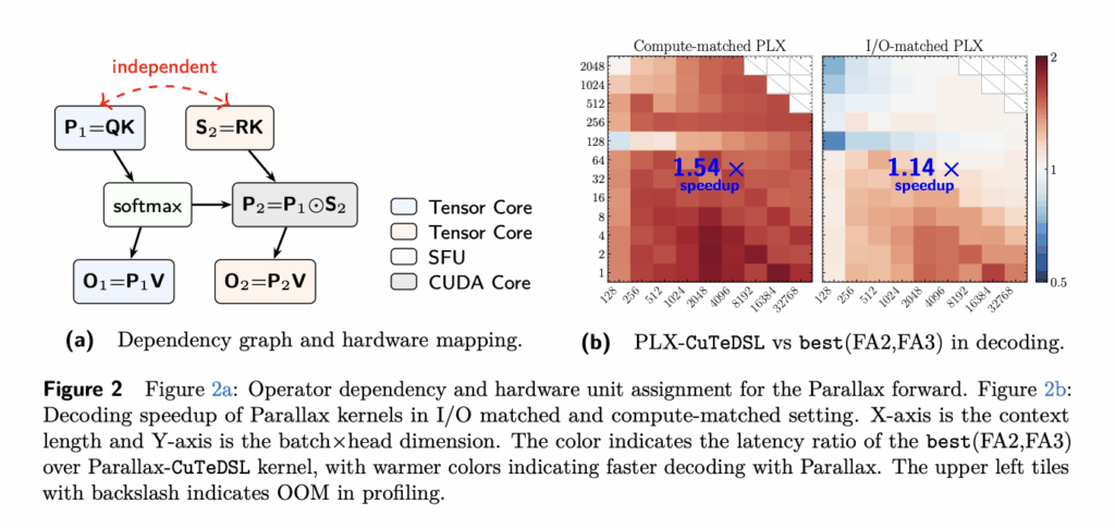
The Transformer’s attention mechanism has barely changed since 2017. Most efficiency work has tried to replace softmax attention outright. A new paper takes a different route. It keeps softmax attention and bolts on a correction branch. A team of researchers from Northwestern University, Tilde Research, and University of Washington introduce a parameterized Local Linear Attention called ‘Parallax’ that scales to LLM pretraining and codesigns with Muon. Parallax does not chase efficiency by cutting compute. It adds compute deliberately, then makes that compute cheaper to run on modern GPUs. What is Parallax Parallax builds on Local Linear Attention (LLA). LLA comes from the test-time regression framework. That framework reads attention as a regression solver over key-value pairs. In this view, keys are training data points. Values are labels. The query is the test point. Softmax attention is a nonparametric estimator called Nadaraya-Watson. It fits a local constant function for each query. LLA upgrades that local constant estimate to a local linear estimate. The research team proves this yields strictly smaller integrated mean squared error. The benefit is better bias-variance tradeoffs for associative memory. But LLA has a problem at scale. Its exact forward requires solving a linear system for every query. That uses a parallel conjugate gradient (CG) solver. The CG solver creates three issues: intensive I/O, a hard regularization-expressiveness tradeoff, and low-precision incompatibility. Parallax removes the solver. Instead, it learns an extra projection matrix. The research team writes this as ρi = WRxi. Here WR is a learnable matrix that probes the KV covariance directly from the layer input. So Parallax keeps the local linear principle. It just replaces the per-query solve with a learned, query-like projector. That makes it simpler, more efficient, and easier to implement. How the Mechanism Works Parallax reformulates LLA as softmax attention plus an additive correction. The output equals the softmax attention output minus a projected covariance term. In the research paper’s notation, that term is the KV covariance multiplied by the learned probe ρi. The research team also drops one piece of LLA called the boundary amplification factor, set to zero. This is necessary for stability. Once the probe is parametric, the original geometric interpretation breaks. Leaving the factor in could cause the scaling to diverge or flip sign. Parallax sits inside a family of attention mechanisms. The research team organizes them in the paper by three axes: the bandwidth, the probe construction, and the affine structure. At one extreme, Parallax degenerates exactly to softmax attention when the probe norm goes to zero. Setting WR = 0 makes a Parallax layer behave identically to softmax attention. So a pretrained Transformer checkpoint can be converted by adding WR and fine-tuning. The Hardware Argument Parallax inherits the streaming structure of FlashAttention. It adds one covariance branch that reuses the same key-value stream. The research team expands the forward into two parallel scoring branches. Both branches share the online maximum, the rescaling factor, and the K and V tiles. So Parallax needs no extra I/O per iteration. The key property is higher arithmetic intensity (AI). AI is the ratio of floating point operations to high-bandwidth memory traffic. In the regime where KV work dominates, Parallax roughly doubles the arithmetic intensity. It adds compute while reusing the same memory stream. This shifts attention toward a more compute-bound regime. That is exactly the regime where kernel optimization helps on modern hardware. The research team prototyped a decode kernel in CuTeDSL on NVIDIA Hopper GPUs. Hopper’s tensor core matmul instructions operate on tiles of at least 64 rows. A decode step supplies only one query row. So the QK and RK products can be computed jointly, within instructions standard attention already issues. They profiled against FlashAttention 2 and 3 on H200 GPUs at BF16 precision. They swept batch sizes from 1 to 2,048 and context lengths from 128 to 32,768. The prototype kernel matches or outperforms FlashAttention across all configurations. The below figure annotates speedups of 1.54× in the compute-matched setting and 1.14× in the I/O-matched setting. https://arxiv.org/pdf/2605.29157 What the Experiments Show The research team validated Parallax on synthetic tasks and on LLM pretraining at 0.6B and 1.7B scales. Models used the Qwen-3 architecture in the torchtitan repository. They trained on the Ultra-FineWeb dataset with a 4096 context length. Baselines included softmax attention (Transformer), Mamba, Gated DeltaNet, MesaNet, and Kimi DeltaAttention. On the MAD-Benchmark, Parallax attained the highest overall accuracy at 0.716 average. It consistently improved recall-oriented tasks like In-Context-Recall and Selective-Copying. It stayed competitive on compression and memorization tasks. On language modeling, Parallax with Muon achieved the best perplexity at both scales. It also posted the highest average downstream accuracy. At 1.7B, Parallax scored 62.45 average against the Transformer’s 61.43. Two controls test where the gain comes from. A parameter-matched Transformer closed only a small fraction of the gap. A compute-matched Parallax still beat both baselines. The paper argues this points to the mechanism itself, not extra parameters or compute. The Optimizer Twist A core finding is an optimizer-architecture interaction. Parallax shows a large advantage under Muon. Under AdamW, the advantage shrinks markedly or even disappears. Muon is a recent optimizer for matrix parameters in hidden layers. It uses the polar factor of the momentum buffer, so updates have condition number exactly one. Prior work shows this produces better-conditioned weight matrices. The research team in the paper traces the gap to the correction branch. They define a correction-to-output ratio (COR). Under Muon, COR exceeds 8 in the deepest layers. Under AdamW, it stays below 4. The WR projection is disproportionately affected. Its stable rank collapses under AdamW but stays high under Muon. A gating experiment confirms the pattern. Under AdamW, the model learns to suppress the correction branch rather than use it. The research team call this the first empirical demonstration of strong architecture-optimizer codesign for attention mechanisms. They do not claim Muon with WSD is the optimal recipe. An appendix ablation shows the advantage shrinks during the decay phase. How the Scores Differ Parallax also produces different

Parallax: A Parameterized Local Linear Attention That Keeps Softmax and Adds a Learned Covariance Correction Branch Beitrag lesen »

AI, Committee, Nachrichten, Uncategorized

The Download: China’s brain implant ambitions

This is today’s edition of The Download, our weekday newsletter that provides a daily dose of what’s going on in the world of technology. China has approved the world’s first invasive brain-computer chip—here’s what’s next Sitting in the courtyard of his house in China’s Henan province last October, Dong Hui decided to try holding a pen. Six years after a car accident left him paralyzed from the neck down, he slowly wrote his name, “Thank you,” and the date. The breakthrough was made possible by a brain implant called NEO. In March, it became the world’s first invasive brain-computer interface approved for use beyond clinical trials. The approval is expected to accelerate China’s push to become a global leader in brain implants. Read the full story on how China reached this milestone—and what it means for the future of brain-computer interfaces. —You Xiaoying The must-reads I’ve combed the internet to find you today’s most fun/important/scary/fascinating stories about technology. 1 Nvidia is launching its first AI chip for personal computersThe RTX Spark will power laptops from Dell, HP, Microsoft, and others. (BBC)+ They’re being designed specifically to run AI agents. (WSJ $) + The first devices are set to launch on Windows PCs in the fall. (CNBC)+ The move marks a challenge to Apple and Intel. (FT $) 2 The US is stopping exports of AI chips to Chinese firms abroadIt’s closed a loophole allowing exports to Chinese subsidiaries. (Reuters $)+ Which may have enabled unlicensed access to Nvidia chips. (Al Jazeera)+ Export curbs have led China to redesign its chip industry. (MIT Technology Review) 3 Surgeons have transplanted pig liver and kidneys into a living personThe clinically dead recipient’s organs worked for almost five days. (Nature)+ Pig organs could ease transplant shortages. (Guardian)+ Putin says organ transplants could grant immortality. (MIT Technology Review)  4 The US, Australia, and UK will defend seabed cables with underwater dronesThey’re developing the vehicles via the trilateral AUKUS defense ⁠pact. (CNN)+ Undersea internet cables face growing threats. (BBC) 5 A new study has revealed chatbots’ manipulative ‘dark patterns’ It found they prey on emotions to encourage harmful behavior. (404 Media)+ They can also sway voters better than political ads. (MIT Technology Review) 6 Apple plans to disrupt the traditional glasses marketIts smart glasses target the broader spectacles industry. (Bloomberg $)+ Smart glasses are also gaining traction in warfare. (MIT Technology Review) 7 AI super PACs are dueling over the midtermsSplit between Anthropic and OpenAI, they’re fighting to shape AI regulation. (NYT $) 8 SoftBank has overtaken Toyota as Japan’s most valuable companyThe AI boom pushed SoftBank’s market value above $305 billion. (Bloomberg $)  9 A botnet of more than 17 million devices has been dismantled in EuropeDutch authorities linked the network to a Russian proxy service. (Ars Technica) 10 Tech leaders are uniting around a transhuman vision for AIThey’re working toward a post-human agenda. (Guardian) Quote of the day “It’s just been shoved down their throats in secrecy. And that makes them upset.”  —Legendary environmental activist Erin Brockovich tells “The Jim Acosta Show” why citizens are angry about data centers expanding into their communities.  One More Thing MIKE BELLEME What happens when you donate your body to science Rebecca George doesn’t mind the vultures. At Western Carolina University’s body farm, forensic anthropologists monitor donors—sometimes for years—as they become nothing but bones. Around 20,000 people donate their cadavers to scientific research and education each year. At anatomy labs and body farms, they help train doctors, advance research, and teach scientists more about the human body long after death. But what actually happens after a body is donated? Read the full story to find out. —A.W. Ohlheiser We can still have nice things A place for comfort, fun, and distraction to brighten up your day. (Got any ideas? Drop me a line.) + This map of moments turns the planet into a shared diary.+ Let editors curate your ideal podcast moments with this app.+ Architecture lovers will enjoy this encyclopedia of famous buildings.+ Get in touch with your emotions through this map exploring more than 100 feelings.

The Download: China’s brain implant ambitions Beitrag lesen »

AI, Committee, Nachrichten, Uncategorized

Meet Memory OS: A 6-Layer Open-Source Memory Stack Built on Top of Hermes Agent

Hermes Agent already remembers across sessions. The open-source agent from Nous Research ships with curated memory files and full-text session search. But a new community project argues that built-in memory is too shallow for serious work. A new library named ‘Memory OS‘ has been released under an MIT license by a developer (ClaudioDrews). It stacks six memory layers onto Hermes. It adds a vector database, structured facts, and an auto-curated knowledge wiki. The project is new but it seems to have a good potential and its architecture shows how agent memory can be layered. Memory OS Memory OS is not a Hermes plugin you toggle on. It is a layered system that sits beside Hermes Agent’s own memory. Hermes already provides workspace files and a session database. Memory OS keeps those and adds four more layers above them. The full stack runs locally using Docker, Qdrant, Redis, and Python 3.11+. It works with any LLM provider Hermes supports, including OpenRouter, OpenAI, Anthropic, and Ollama. The README frames it as a “memory operating system,” not a single feature. The Six Layers, From Files to Vectors Layer 1 is Workspace. It holds MEMORY.md, USER.md, and CREATIVE.md, injected into the system prompt each turn. Layer 2 is Sessions. It uses state.db, a SQLite database with FTS5 full-text search across conversation history. Layer 3 is Structured Facts. It stores durable facts in memory_store.db, using SQLite, HRR, FTS5, and trust scoring. A feedback loop adjusts those trust scores over time, alongside entity resolution. Layer 4 is Fabric, a heavily forked version of the Icarus Plugin. This fork adds LLM-powered session extraction over the upstream esaradev/icarus-plugin. It handles cross-session recall through 16 tools, including fabric_recall, fabric_write, and fabric_brief. Layer 5 is the Vector Database, built on Qdrant. It uses 4096d Cosine vectors plus BM25 sparse search, a keyword-style ranking method. Layer 6 is an LLM Wiki, an auto-curated vault of concepts, entities, and comparisons. That wiki is continuously ingested back into Qdrant through a process called wiki-continuous-ingest. How the Retrieval Flow Works The flow sits on when memory is read and written. On pre_llm_call, Memory OS runs what it calls surgical recall. It pulls from four sources at once: Fabric, Qdrant, Sessions, and Facts. Each source is gated by a relevance threshold before anything reaches the model. Per-session deduplication stops the same context from appearing twice. A social-closer filter skips trivial messages, such as a plain “thanks.” On post_llm_call and on_session_end, the system extracts and captures new learnings automatically. The stated goal is token efficiency, not stuffing the context window. The Fallback Cascade and Cleanup Layer 5’s retrieval uses a four-level fallback. It tries hybrid search first, then dense vectors, then lexical, then SQLite. If one method fails or returns nothing, the next takes over. This design keeps recall working even when the vector database struggles. Memory OS also runs a weekly decay scanner to age out stale entries. Semantic dedup merges near-identical memories when cosine similarity exceeds 0.92. These housekeeping steps aim to stop memory from bloating over months of use. Local-First, And Deliberately So Memory OS positions itself against cloud memory services like mem0, Zep, and Letta. Its pitch is that memory infrastructure should run on your own machine. The memory data stays local, with no memory subscription. LLM calls still go to whichever provider you choose. Hermes itself already supports eight external memory providers, including mem0 and Honcho. Memory OS is not one of those official providers. It is a separate, community-built stack layered on Hermes directly. For teams with data-residency rules, a local memory store can matter. Just open-sourced **Memory OS** — a complete hierarchical persistent memory architecture for the Hermes Agent. 6 layers, fully local:• Structured facts + trust scoring with feedback loop• Hybrid vector search (Qdrant + BM25)• Self-curating LLM Wiki• Semantic… — Claudio Drews (@ClaudioDrews25) May 31, 2026 Strengths and Limitations Strengths: Clear layered design separating files, sessions, facts, vectors, and a wiki Fully local infrastructure with no cloud memory subscription Provider-agnostic, matching Hermes Agent’s own flexibility Token-efficient retrieval by design, via gated sources and per-session deduplication Limitations: Brand new, with few commits A forked Icarus Plugin that the author says is not upstream-compatible Heavier setup: Docker, Qdrant, Redis, and an ARQ Worker all required No published benchmarks on recall quality, latency, or token savings Key Takeaways Memory OS is a community-built, MIT-licensed stack that adds six memory layers on top of Hermes Agent. It combines workspace files, FTS5 session search, trust-scored facts, a forked Icarus fabric, Qdrant vectors, and an auto-curated LLM wiki. Retrieval runs on pre_llm_call with gated, deduplicated recall from four sources; capture runs on post_llm_call and on_session_end. Memory infrastructure is fully local and provider-agnostic, but LLM calls still go to your chosen provider. Check out the Repo. Also, feel free to follow us on Twitter and don’t forget to join our 150k+ ML SubReddit and Subscribe to our Newsletter. Wait! are you on telegram? now you can join us on telegram as well. Need to partner with us for promoting your GitHub Repo OR Hugging Face Page OR Product Release OR Webinar etc.? Connect with us The post Meet Memory OS: A 6-Layer Open-Source Memory Stack Built on Top of Hermes Agent appeared first on MarkTechPost.

Meet Memory OS: A 6-Layer Open-Source Memory Stack Built on Top of Hermes Agent Beitrag lesen »

AI, Committee, Nachrichten, Uncategorized

Trajectory Releases a Concurrent Multi-LoRA Training Stack for Continual Learning, Reporting a 2.81× Experiment-Throughput Gain

Trajectory’s concurrent multi-LoRA stack reports a 2.81× experiment-throughput gain over single-tenant RL, with all code in the NovaSky-AI/SkyRL GitHub repository. Most language models improve in discontinuous jumps. A team collects data, trains, and ships a new version. This takes months and produces remarkable or catastrophic behavior for users. Trajectory wants to replace that cycle with continual learning. The Trajectory team published a field report describing how. It built a concurrent, multi-LoRA training platform for continuously learning workloads. The work was done with UC Berkeley Sky Lab and Anyscale. All training code is open-sourced in the NovaSky-AI/SkyRL repository. The result is a 2.81× end-to-end experiment-throughput improvement. The comparison is against a single-tenant training framework. Trajectory reports no regression on any training rewards. What Multi-LoRA Training Actually Is Continual learning requires models to update from live feedback and production interactions. A coding agent could learn engineering patterns as developers correct its work. A support agent could resolve hard tickets as operators intervene on difficult cases. Most training infrastructure still assumes a linear lifecycle. Teams allocate GPUs, initialize the model, run a job, then spin down. Continual learning revises that relationship. When production interactions become training inputs, training becomes part of a live system. Modern RL training reduces to three core primitives. The Sampler generates trajectories from the current policy model. The Trainer computes gradients and updates the policy weights. Parameter synchronization broadcasts updated weights back to inference workers. Trajectory calls its approach Continuous Multi-LoRA Training, or C-LoRA. Each experiment maps to a dedicated LoRA adapter on a warm, multi-tenant engine. The Problems It Targets The Trajectory team identifies four inefficiencies in traditional stacks: (1) Cold starts are slow: Every serial job reloads checkpoints, initializes the distributed runtime, and warms inference engines. For large models, this step alone can exceed 30 minutes per run. (2) RL is memory intensive: Frontier models often exceed 100B parameters. Qwen3.5-397B can require up to eight H200 nodes to fit into memory. LoRA cuts memory usage by an order of magnitude. It freezes the base model and trains only small adapter weights. (3) Traditional stacks are single-tenant: They run one experiment at a time. Multi-LoRA maps each experiment to one adapter, multiplexing throughput by a factor of N. (4) Job utilization is low: Trainers and inference engines stall while waiting for each other. Multi-LoRA load balances across jobs to fill idle capacity. Inside the Architecture Most throughput wins come from inference. In vLLM, all adapters are hot-loaded in GPU memory. Decode steps can then mix tokens from different adapters in the same batch. The key enabler is the SGMV decode kernel. It fuses per-adapter matrix-vector work into one GPU launch per decode step. After each optimization step, updated LoRA weights load in-place into the inference engine. The scheduler does not freeze, so other tenants keep decoding. Training works differently. One active LoRA adapter trains on the GPU. The rest sit in pinned CPU memory. Each tenant’s state lives in an AdapterStore. It holds LoRA parameters, FP32 master weights, optimizer moments, and gradient buffers. The engine swaps one tenant’s state onto the GPU, runs a single forward_backward pass, then swaps it back. This training path is still single-adapter. The inference concurrency gains do not yet apply to training. The Numbers Trajectory tested on a single H200 node with Qwen3-4B-Instruct-2507. It ran sync RL on GSM8K in an agentic setting. The Trajectory team reframed GSM8K as a tool use learning task. The model decides when to call a Calculator and a Final Answer tool. Reward is 1.0 only when Final Answer is called with the correct answer. The policy starts near 40% accuracy at step 0. With the right learning algorithm, it climbs past 90% by step 9. The Trajectory team scaled to eight concurrent multi-LoRA runs. Final Experiment Time hit 5433s at N=8, a 2.81× speedup. Eight concurrent experiments finished before three serial runs back-to-back. Mean Experiment Time also improved, peaking at N=4 with a 1.88× speedup. Every concurrency level reached reward_accuracy above 90% by step 9. The Tradeoffs Higher throughput costs per-step latency. As N grows, First Experiment Time and Step Time degrade. At N=8, the first serial experiment finishes 1.97× faster. Mean step time rises from 191s to 500s, only 2.62× slower. Most of that increase is rollout time. Rollout grows from 162s to 401s, roughly 77% of the increase. At N=2, doubling the load adds only 15% rollout time. That is the ideal case for multi-LoRA. The pattern held on a harder workload. On τ-bench retail with the NVIDIA-Nemotron-3-Nano-30B-A3B-BF16 MoE model, N=2 finished 10 steps 1.28× faster. Per-tenant step time rose 1.57×. Strengths and Weaknesses Strengths: 2.81× end-to-end experiment-throughput gain at eight concurrent runs No accuracy regression; runs tracked the serial baseline within ±1σ in the final steps LoRA cuts memory by an order of magnitude versus full fine-tuning Fully open-sourced in NovaSky-AI/SkyRL for the community to build on Weaknesses: Per-step latency and First Experiment Time degrade as N grows Training remains serialized across tenants; only inference is multiplexed Tested mainly on mid-sized models, not frontier-scale parameters Setup requires an 8× H100/H200 node and a Megatron build Key Takeaways Trajectory built a concurrent, multi-LoRA RL training stack for continual learning, open-sourced in NovaSky-AI/SkyRL. It reports a 2.81× end-to-end experiment-throughput gain over a single-tenant baseline, with no reward regression. Each experiment maps to a dedicated LoRA adapter on an always-hot engine, multiplexing throughput by N. Most gains come from vLLM multi-LoRA inference via the SGMV decode kernel; training stays single-adapter. The tradeoff is per-step latency: at N=8, step time rises from 191s to 500s. Marktechpost’s Visual Explainer Field Report · May 27, 2026 Continuous Multi-LoRA Training for Continual Learning Trajectory, built with UC Berkeley Sky Lab and Anyscale. 2.81× end-to-end experiment-throughput gain Training code open-sourced in the NovaSky-AI/SkyRL repository. 01 — What it is One always-hot engine, many adapters Continual learning updates models from live feedback and production interactions. Trajectory calls its approach Continuous Multi-LoRA Training (C-LoRA). Each experiment maps to a dedicated LoRA adapter on

Trajectory Releases a Concurrent Multi-LoRA Training Stack for Continual Learning, Reporting a 2.81× Experiment-Throughput Gain Beitrag lesen »

AI, Committee, Nachrichten, Uncategorized

Best Text-to-Speech TTS Models in 2026: A Benchmark-Based Comparison

Text-to-speech TTS moved fast over the past year. The line between synthetic and human speech narrowed. Latency dropped below 100 milliseconds for some real-time systems. Emotional control became a standard feature rather than a research demo. This guide reviews the models that really matter in 2026. It is written for AI professionals choosing a model for production. How to read TTS benchmarks in 2026 Two benchmarks dominate in most community discussions. The first is the Artificial Analysis Speech Arena Leaderboard. It ranks models by blind human preference using an ELO rating. As of 2026 it evaluates dozens of production APIs. The second is the community-run TTS Arena on Hugging Face. It uses the same blind A/B voting method. These leaderboards measure perceived quality, not accuracy. They also change continuously. As of May 30, 2026, the Artificial Analysis Speech Arena lists Gemini 3.1 Flash TTS, Realtime TTS-2 (Research Preview), Sonic 3.5, Realtime TTS 1.5 Max, and Fun-Realtime-TTS-Preview as its top five by ELO. Those positions shifted within the prior weeks, and they will shift again. Treat any single number as a point-in-time reading, not a fixed truth. Accuracy needs separate measurement. Trelis Research tested ten models using a round-trip character error rate, or CER. The method transcribes generated audio with an ASR model, then compares it to the input text. Mean opinion score, or MOS, captures perceived naturalness. Both metrics have limits. Round-trip CER depends on the ASR model’s own accuracy. The UTMOS quality estimator was trained on audio up to ten seconds, so longer samples show less score spread. Latency is the third axis. The relevant figure for voice agents is time-to-first-audio, or TTFA. Time-to-first-byte, or TTFB, can be misleading, since container headers carry no audio. Consistency matters as much as the median. A Gradium benchmark from May 2026 measured the interquartile range across providers. Tail latency, not the average, determines user experience at scale. In short, no benchmark is complete. Quality, accuracy, latency, language coverage, and price all trade off. The right model depends on which axis your application cannot compromise. Commercial leaders #1 Inworld TTS-1.5 and Realtime TTS-2 Inworld AI is a research lab founded by a team from Google and DeepMind. It released TTS-1.5 on January 21, 2026. The model targets real-time, consumer-scale applications. Inworld reports roughly 30 percent more expressive range than TTS-1. It also reports about 40 percent better stability, measured through word error rate and output consistency. TTS-1.5 ships in two tiers. The Mini tier is tuned for latency-sensitive workloads such as voice agents and gaming. The Max tier balances higher stability with low latency. Inworld reports P90 time-to-first-audio under 130 milliseconds for Mini and under 250 milliseconds for Max. The model supports 15 languages and offers both instant and professional voice cloning. Pricing is tiered by plan, not a single rate. On the On-Demand and Creator plans, Inworld lists $25 per million characters for TTS 1.5 Mini and $35 for Realtime TTS-2 and TTS 1.5 Max. The Developer and Growth plans cut those rates; Growth reaches $15 for Mini and $25 for Max and TTS-2. Enterprise pricing goes as low as $5 and $10 respectively. Note that TTS 1.5 covers 15 languages, while TTS-2 covers over 100. Inworld later added Realtime TTS-2 in 2026. It is described as a closed-loop voice model with stronger steering and expressiveness. Across several leaderboard snapshots, Inworld reported holding three of the top five spots on the Artificial Analysis Speech Arena. Inworld suits developers building voice agents at consumer scale. The combination of low latency and aggressive pricing is its main draw. #2 Google Gemini 3.1 Flash TTS Google DeepMind released Gemini 3.1 Flash TTS on April 15, 2026. It is a preview model available through the Gemini API, Google AI Studio, Vertex AI, and Google Vids. The model introduces more than 200 audio tags. These tags steer style, tone, pacing, accent, and scene direction. On Google’s own report, the model reached an ELO of 1,211 on the Artificial Analysis leaderboard. It supports 70-plus languages and native multi-speaker dialogue. Google built it on the Gemini family rather than a standalone speech stack. The model treats generation as a language task: it decides not only what to say, but how to say it. The model has documented limitations that matter for deployment. A TTS session has a 32,000-token context window, and Google’s docs state that Gemini TTS does not support streaming. It is built for controlled text recitation, not interactive voice agents; the separate Live API is Google’s real-time path. Output quality can drift on generations longer than a few minutes, so Google recommends chunking. The model offers 30 prebuilt voices. All generated audio carries a SynthID watermark for AI-content identification. Gemini 3.1 Flash TTS fits podcast and audiobook generation with fine-grained control. It is a strong default for teams already on Google Cloud. #3 ElevenLabs v3 ElevenLabs released Eleven v3 in alpha on June 5, 2025. It reached general availability in early 2026, per the company’s announcement. ElevenLabs describes it as its most expressive model. It introduced inline audio tags formatted in lowercase square brackets. Examples include [whispers], [laughs], [sighs], and scene cues like [interrupting]. The model supports more than 70 languages. The GA release refined the alpha. ElevenLabs reports users preferred the new version about 72 percent of the time. It also improved how the model handles numbers, symbols, and specialized notation. A key feature is Text to Dialogue. It weaves multiple voices into one generation pass. The model matches prosody and emotional range across speakers. It can handle interruptions and shifting moods with limited prompting. Eleven v3 still requires more prompt engineering than earlier models. It is not built for real-time use. ElevenLabs states the larger model and higher-fidelity codec take longer to run. For real-time and conversational use, the company recommends Flash v2.5 instead. Those models stream with low latency, around the 75-millisecond range in vendor figures. ElevenLabs v3 fits narrative content, audiobooks, and character work where quality outweighs speed. It remains a common

Best Text-to-Speech TTS Models in 2026: A Benchmark-Based Comparison Beitrag lesen »

AI, Committee, Nachrichten, Uncategorized

A Coding Implementation on Loguru for Designing Robust, Structured, Concurrent, and Production-Ready Python Logging Pipelines

In this tutorial, we implement a practical use case with Loguru, a powerful, flexible, and production-ready logging library for Python. We start by building a clean, idempotent logging setup that can be safely rerun without duplicating handlers or producing messy output. From there, we move step by step through structured logging, contextual logging, custom log levels, global patching, callable formatters, and in-memory sinks. We also handle real-world logging needs such as rich exception traces, JSON log files, custom rotation, compression, retention, async logging, threaded execution, multiprocessing-safe logging, and standard logging module interception. By keeping everything in a Colab-ready workflow, we make it easy to test, inspect, and understand how Loguru can support debugging, monitoring, and observability in serious Python applications. Copy CodeCopiedUse a different Browser !pip install -q loguru nest_asyncio import os, sys, time, json, glob, gzip, shutil, asyncio, logging, itertools, multiprocessing from collections import deque from concurrent.futures import ThreadPoolExecutor, ProcessPoolExecutor from loguru import logger try: import nest_asyncio; nest_asyncio.apply() except Exception as e: print(“nest_asyncio not applied:”, e) WORKDIR = “/content/loguru_demo” if os.path.isdir(“/content”) else “/tmp/loguru_demo” os.makedirs(WORKDIR, exist_ok=True); os.chdir(WORKDIR) for f in glob.glob(“*”): try: os.remove(f) except OSError: pass print(f”Working directory: {WORKDIR}n”) RESULTS = [] def check(name, condition, detail=””): ok = bool(condition); RESULTS.append((name, ok)) print(f” [{‘PASS’ if ok else ‘FAIL’}] {name}” + (f” — {detail}” if detail else “”)) def banner(t): print(f”n{‘=’*64}n {t}n{‘=’*64}”) _seq = itertools.count(1) def global_patcher(record): record[“extra”].setdefault(“env”, “colab”) record[“extra”][“seq”] = next(_seq) _NOISE = {“env”, “seq”, “app”} def console_formatter(record): fmt = (“<green>{time:HH:mm:ss.SSS}</green> | <level>{level: <8}</level> | ” “<cyan>{name}:{function}:{line}</cyan> – <level>{message}</level>”) if any(k not in _NOISE for k in record[“extra”]): fmt += ” | <yellow>{extra}</yellow>” return fmt + “n{exception}” We install Loguru and supporting dependencies, import all required libraries, and prepare a clean working directory for the tutorial. We also create a small verification helper to test each feature as the tutorial runs. We then define a global patcher and console formatter so that every log record carries useful metadata and appears in a readable format. Copy CodeCopiedUse a different Browser class MemorySink: def __init__(self, capacity=2000): self.buffer = deque(maxlen=capacity) def write(self, message): self.buffer.append(message.record) def flush(self): pass def has_level(self, name): return any(r[“level”].name == name for r in self.buffer) def find(self, pred): return [r for r in self.buffer if pred(r)] MAX_BYTES = 1500 def size_rotation(message, file): return file.tell() + len(message) > MAX_BYTES def gzip_compression(filepath): with open(filepath, “rb”) as fi, gzip.open(filepath + “.gz”, “wb”) as fo: shutil.copyfileobj(fi, fo) os.remove(filepath) def keep_latest_retention(files): for old in sorted(files, key=os.path.getmtime, reverse=True)[3:]: try: os.remove(old) except OSError: pass class InterceptHandler(logging.Handler): def emit(self, record): try: level = logger.level(record.levelname).name except ValueError: level = record.levelno frame, depth = logging.currentframe(), 2 while frame and frame.f_code.co_filename == logging.__file__: frame, depth = frame.f_back, depth + 1 (logger.opt(depth=depth, exception=record.exc_info) .bind(stdlib_logger=record.name) .log(level, record.getMessage())) def mp_worker(n): logger.bind(child=os.getpid()).info(“hello from child item {}”, n) return os.getpid() We create reusable logging components that make the tutorial more practical and production-like. We define an in-memory sink, custom file rotation, compression, and retention functions to control how logs are stored. We also built a standard logging interceptor and a multiprocessing worker to connect Loguru to external libraries and child processes. Copy CodeCopiedUse a different Browser banner(“1) logger.configure(): handlers + custom level + extra + patcher”) mem = MemorySink() logger.configure( handlers=[ {“sink”: sys.stderr, “format”: console_formatter, “level”: “DEBUG”, “colorize”: True, “backtrace”: True, “diagnose”: True}, {“sink”: mem, “level”: “DEBUG”, “format”: “{message}”}, {“sink”: “structured.jsonl”, “serialize”: True, “level”: “DEBUG”, “enqueue”: True}, {“sink”: “errors.log”, “level”: “ERROR”, “enqueue”: True, “backtrace”: True, “diagnose”: False, “format”: “{time:YYYY-MM-DD HH:mm:ss} | {level} | ” “{name}:{function}:{line} | {message}”}, ], levels=[{“name”: “NOTICE”, “no”: 22, “color”: “<blue><bold>”, “icon”: “”}], extra={“app”: “loguru-advanced”}, patcher=global_patcher, ) logger.debug(“debug”); logger.info(“info”); logger.success(“SUCCESS level ships built-in”) logger.warning(“warning”); logger.log(“NOTICE”, “custom level between INFO and SUCCESS”) banner(“2) bind() / contextualize() / patch()”) logger.bind(user_id=42, request_id=”abc-123″).info(“bound context”) with logger.contextualize(task=”batch-job”, run=7): logger.info(“inside contextualized block”) logger.patch(lambda r: r[“extra”].update(epoch=round(time.time()))).info(“per-call patched record”) banner(“3) @logger.catch + context-manager form”) def inner(d): return d[“a”] / d[“b”] def outer(d): return inner(d) @logger.catch(reraise=False) def compute(d): return outer(d) compute({“a”: 1, “b”: 0}) with logger.catch(message=”handled inside a with-block”): raise ValueError(“boom in block”) banner(“4) opt(lazy=True), inline colors, record access”) logger.opt(lazy=True).debug(“lazy sum = {}”, lambda: sum(i*i for i in range(1_000_000))) logger.opt(colors=True).info(“inline <red>colors</red> <green>work</green>”) logger.opt(record=True).info(“emitted from source line {record[line]}”) We configure Loguru with multiple handlers, including console output, memory capture, JSON logging, and error logging. We then demonstrate structured logging with bound context, contextual blocks, patched records, and a custom log level. We also explore exception handling and useful opt() features such as lazy evaluation, inline colors, and record access. Copy CodeCopiedUse a different Browser banner(“5) custom rotation/compression/retention (forces real rotation)”) ev_id = logger.add(“events_{time:HHmmss_SSS}.log”, rotation=size_rotation, compression=gzip_compression, retention=keep_latest_retention, enqueue=True, level=”DEBUG”, format=”{time:HH:mm:ss.SSS} | {level: <8} | {message}”) for i in range(80): logger.bind(idx=i).debug(“rotating event line number {}”, i) logger.complete(); logger.remove(ev_id) print(f” archives created: {sorted(glob.glob(‘events_*.gz’))}”) banner(“6a) ThreadPoolExecutor with per-thread contextualize()”) thread_caps = [] tid = logger.add(thread_caps.append, level=”DEBUG”, format=”{message}”, filter=lambda r: “worker_id” in r[“extra”]) def worker(n): with logger.contextualize(worker_id=n): logger.info(“thread work item {}”, n) return n * n with ThreadPoolExecutor(max_workers=8) as ex: sq = list(ex.map(worker, range(8))) logger.complete(); logger.remove(tid) worker_ids = {m.record[“extra”][“worker_id”] for m in thread_caps} banner(“6b) async coroutine sink + await logger.complete()”) async def run_async_demo(): sunk = [] async def async_sink(message): await asyncio.sleep(0); sunk.append(message.record[“message”]) sid = logger.add(async_sink, level=”DEBUG”, catch=True) async def task(n): with logger.contextualize(coro=n): logger.info(“async task {} start”, n) await asyncio.sleep(0.01) logger.success(“async task {} done”, n) await asyncio.gather(*(task(i) for i in range(5))) await logger.complete() logger.remove(sid) return sunk try: async_msgs = asyncio.run(run_async_demo()) except RuntimeError: async_msgs = asyncio.get_event_loop().run_until_complete(run_async_demo()) print(f” async sink received {len(async_msgs)} messages”) We demonstrate custom file management by automatically rotating, compressing, and retaining log files. We then test thread-safe logging by running multiple workers, each with its own contextual metadata. We also add an asynchronous coroutine sink to see how Loguru handles async tasks and correctly drains pending logs. Copy CodeCopiedUse a different Browser banner(“7) intercept stdlib `logging` and filter a chatty library”) logging.basicConfig(handlers=[InterceptHandler()], level=0, force=True) lib_caps = [] def lib_filter(record): if record[“extra”].get(“stdlib_logger”) == “chatty”: return record[“level”].no >= logger.level(“WARNING”).no return True lid = logger.add(lib_caps.append, level=”DEBUG”, format=”{message}”, filter=lambda r: (“stdlib_logger” in r[“extra”]) and lib_filter(r)) logging.getLogger(“chatty”).info(“noisy info (should be filtered out)”) logging.getLogger(“chatty”).warning(“noisy warning (kept)”) logging.getLogger(“important”).debug(“important debug (kept)”) logger.complete(); logger.remove(lid) banner(“8) SELF-TESTS”) logger.complete(); time.sleep(0.2) try: rec = json.loads(open(“structured.jsonl”).read().splitlines()[-1]) check(“JSON sink serializes records”, {“text”,

A Coding Implementation on Loguru for Designing Robust, Structured, Concurrent, and Production-Ready Python Logging Pipelines Beitrag lesen »

AI, Committee, Nachrichten, Uncategorized

StepFun Releases Step 3.7 Flash: A 198B MoE Vision-Language Model for Coding Agents and Search Workflows

StepFun today released Step 3.7 Flash, a multimodal Mixture-of-Experts model targeting agentic use cases. It adds native vision input and improved tool-use reliability over Step 3.5 Flash. What is Step 3.7 Flash? Step 3.7 Flash is a 198B-parameter sparse Mixture-of-Experts (MoE) vision-language model. It pairs a 196B-parameter language backbone with a 1.8B-parameter vision encoder (ViT) for native image understanding. The model activates approximately 11B parameters per token during inference. In MoE architectures, only a subset of “expert” sub-networks fires per forward pass — not the full network. This keeps inference compute closer to an 11B dense model while maintaining a 198B total parameter budget. Key specs: Spec Value Total parameters 198B (196B language + 1.8B ViT) Active parameters per token ~11B Context window 256k tokens Throughput Up to 400 tokens/sec Reasoning levels Low, medium, high License Apache 2.0 Architecture Notes The vision encoder runs as a separate 1.8B ViT module. It injects image representations into the language backbone’s context. Step 3.5 Flash had no multimodal support; this is a new addition in 3.7. Three selectable reasoning depths — low, medium, and high — let developers trade latency for reasoning depth. Low is faster and cheaper; high applies more computation per response. Agentic Coding Performance On SWE-Bench Pro, Step 3.7 Flash scores 56.26%, up from Step 3.5 Flash’s 51.3% — a gain of roughly 5 percentage points. On Terminal-Bench 2.1, it scores 59.55%, up from 53.37%. On SWE-MTLG (a multi-task long-generation coding benchmark), it scores 72.42%. Cross-harness consistency on StepFun’s internal Step-SWE-Bench: Scaffold Step 3.7 Flash Step 3.5 Flash Hermes Agent 67.5% 60.0% OpenClaw 67.0% 47.0% KiloCode 67.5% 59.0% RooCode 64.5% 43.0% Claude Code 71.5% 73.0% OpenCode 64.5% 57.0% Step 3.5 Flash ranged from 43% to 73% across harnesses. Step 3.7 Flash ranges from 64.5% to 71.5%. In production, coding agents often run inside heterogeneous scaffolds — each with its own prompting conventions and tool schemas. Narrower per-harness variance means more predictable behavior across different setups. Advisor Mode Step 3.7 Flash supports Advisor Mode, StepFun’s implementation of the advisor strategy described by Anthropic. The model runs the agentic loop end-to-end — calling tools, reading results, iterating — and escalates to a larger advisor model only at specific inflection points, such as planning or recovering from repeated failures. Most of the run stays at executor cost. With Advisor Mode enabled on SWE-Bench Verified, StepFun reports Step 3.7 Flash reaches 97% of Claude Opus 4.6’s coding performance at roughly one-ninth the per-task cost ($0.19 vs. $1.76 per task). These are StepFun’s internal figures. Multimodal Capabilities Step 3.7 Flash supports two visual tool pathways: Visual Search Tool — For recognition tasks where the model’s parametric knowledge is insufficient (long-tail entities, recently emerged concepts), it invokes a visual search tool to retrieve and verify. On SimpleVQA (with Search), it scores 79.16%, comparable to GPT 5.5 (79.11%) and above Kimi K2.6 (78.24%) and GLM 5V Turbo (78.20%). Python Tool — For fine-grained visual tasks (high-resolution images, visual probing, bounding-box analysis), it uses a code interface to crop, zoom, and draw pixels or bounding boxes. On V (a self-tested score with Python), it scores 95.29%. On HR-Bench 4K and HR-Bench 8K, it scores 89.13% and 86.34% respectively. StepFun notes an observed behavior during testing: the model combined visual tools with non-visual tools without being explicitly trained to do so. For example, after generating frontend code, it used the GUI to render and inspect the result before iterating. StepFun describes this as emergent compositional tool use. On Android Daily (long-horizon phone UI task completion), Step 3.7 Flash scores 61.87%, ahead of Kimi K2.6 (53.36%) and GLM 5V Turbo (51.68%). Gemini 3 Flash (63.21%) leads this benchmark. Search and Research Benchmarks StepFun focused this model’s search design on planning, evidence filtering, and synthesis — integrating search as part of the reasoning loop rather than a separate add-on. Benchmark Step 3.7 Flash Notable comparison HLE with Tools (acc) 47.20% DeepSeek V4 Flash: 45.10% BrowseComp (acc) 75.82% Claude Opus 4.7: 79.30% DeepSearchQA (F1) 92.82% Kimi K2.6: 92.50% ResearchRubrics (score) 71.68% GPT 5.5: 61.50% Note: The HLE with Tools score of 47.20% compares to Step 3.5 Flash’s text-only score of 35.68%. Step 3.5 Flash did not support tool-augmented evaluation on HLE. General Agent Benchmarks Benchmark Step 3.7 Flash Description Toolathlon 49.51% Multi-tool coordination ClawEval-1.1 67.07% Daily autonomous task execution in realistic environments GDPval (44 occupations) 45.8% General professional task execution Tau2-bench Telecom >98% Across different reasoning difficulty tiers On ClawEval-1.1, Step 3.7 Flash (67.07%) leads DeepSeek V4 Flash (57.80%) and DeepSeek V4 Pro (59.80%) among the compared models. Long-Context Performance On AA-LCR (a long-context retrieval benchmark, avg@16/acc), Step 3.7 Flash scores 63.94%. This is comparable to DeepSeek V4 Flash (63.70%) and DeepSeek V4 Pro (66.30%). Pricing Token Type Price Input (cache miss) $0.20 / M tokens Input (cache hit) $0.04 / M tokens Output $1.15 / M tokens Marktechpost’s Visual Explainer Model Release Step 3.7 Flash — A 198B MoE Vision-Language Model StepFun · Released May 29, 2026 · Apache 2.0 Slide 1 of 8 — Overview What Is Step 3.7 Flash? Step 3.7 Flash is a sparse Mixture-of-Experts (MoE) vision-language model from StepFun. It combines a 196B-parameter language backbone with a 1.8B-parameter Vision Transformer (ViT) encoder for native image understanding. In a MoE model, only a subset of “expert” sub-networks activates per token — not the full network. This keeps inference compute close to an 11B dense model while maintaining 198B total parameters. Total Params 198B Active / Token ~11B Context Window 256k tokens Throughput 400 tok/sec Reasoning Levels Low / Med / High License Apache 2.0 Slide 2 of 8 — Architecture Architecture Notes The 1.8B ViT encoder runs as a separate module and injects image representations into the language backbone’s context. Step 3.5 Flash was text-only; native multimodal support is new in 3.7. Three selectable reasoning depths let developers balance speed and cost: Low — Fastest, cheapest. Suitable for simple completions. Medium — Balanced cost and reasoning depth. High — More compute per response. Best for complex agent

StepFun Releases Step 3.7 Flash: A 198B MoE Vision-Language Model for Coding Agents and Search Workflows Beitrag lesen »

AI, Committee, Nachrichten, Uncategorized

NVIDIA Introduces X-Token: Projection-Guided Cross-Tokenizer KD That Outperforms GOLD by +3.82 Average Points on Llama-3.2-1B

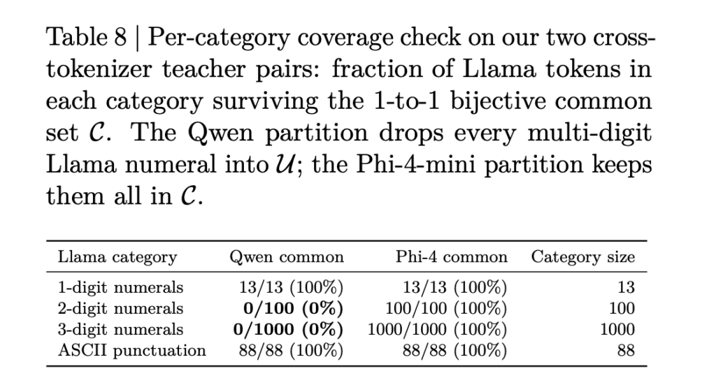
Knowledge distillation (KD) transfers “dark knowledge” from a large teacher model to a smaller student. The student learns from the teacher’s full output probability distribution over tokens, not just correct answers. This is done via per-position Kullback–Leibler (KL) divergence over next-token probability distributions. This formulation requires a shared tokenizer. A practitioner committed to Llama-3.2-1B cannot leverage stronger teachers with incompatible tokenizers — such as Phi-4-mini or Qwen3-4B — because token positions do not correspond across vocabularies. This also prevents multi-teacher distillation across tokenizer families. NVIDIA researchers introduced X-Token, a logit-distribution-based method for cross-tokenizer KD (Knowledge distillation). It operates as a drop-in replacement for the standard KD loss, requiring no auxiliary trainable components and no architectural changes. The Problem X-Token is Solving Two prior approaches dominate cross-tokenizer KD. ULD (Universal Logit Distillation) sidesteps vocabulary alignment by rank-sorting both distributions and minimizing L1 distance. It discards token identity entirely. GOLD adds span alignment and a hybrid loss. It partitions tokens into a 1-to-1 string-matched common subset, trained with KL divergence, and an uncommon remainder, trained with ULD-style rank matching. GOLD is the current state of the art. The research team identifies two structural failures in GOLD’s design: Failure 1: Uncommon-token failure– When tokenizers fragment text differently, critical tokens fall into the unmatched uncommon subset. Llama-3 packs multi-digit numbers as single tokens — “201” is one token. Qwen3 splits them digit by digit: “2”, “0”, “1”. Under GOLD, all 1,100 of Llama’s two- and three-digit numerals (100 two-digit, 1,000 three-digit) fall into the uncommon set when Qwen3-4B is the teacher. Those tokens receive two types of harmful signal: identity-agnostic noise from rank-based ULD matching, and suppressive gradients from the common-KL term acting through the full-vocabulary softmax. The result: GSM8k accuracy drops to 2.56 under GOLD with Qwen3-4B, compared to 12.89 for same-tokenizer KD from a weaker Llama-3.2-3B teacher. Failure 2: Over-conservative matching– GOLD uses strict string equality to define the common subset. A student token Hundreds corresponds to teacher tokens Hund followed by reds under teacher-side re-tokenization, but strict matching discards this pair. Useful alignment signal is lost even when the correspondence is well-formed. These two failures require opposite remedies: eliminate the partition when critical tokens are misaligned, and relax it when alignment is structurally sound. How X-Token Works X-Token has three components: span alignment, a projection matrix W, and two complementary loss formulations — P-KL and H-KL. Span Alignment Teacher and student tokenizers produce sequences of different lengths for the same text. X-Token uses dynamic-programming (DP) span alignment, grouping tokens into chunks where each chunk-pair decodes to the same underlying text substring. A chain-rule merge then combines per-token probabilities within each chunk into a single chunk-level distribution for use in the distillation loss. The alignment is cached per sequence and adds no per-step training overhead. The research team also identifies a failure in TRL’s surface-substring alignment, which is used in TRL’s GOLD trainer. TRL accumulates per-side decoded buffers and flushes only when both buffers match as equal raw strings. A byte-level disagreement — such as Llama-3 auto-prepending <bos> while Qwen-3 does not — prevents future flushes and forces all remaining tokens into one mis-grouped super-group at end of sequence. The DP approach handles this with a single gap move, regardless of sequence length. The Projection Matrix W After alignment, teacher and student distributions still operate over different vocabularies. The projection matrix W ∈ ℝVS|×|VT| maps each student token to a weighted combination of teacher tokens, bridging the vocabulary mismatch. W is constructed deterministically in two passes: Pass 1 (exact-match): For every (student token, teacher token) pair whose decoded strings match after canonicalization, set W[s, t] = 1. Canonicalization unifies space prefixes (Ġ, _, ␣), newlines, byte-fallback tokens of the form <0xHH>, and model-specific special tokens across tokenizer families. Pass 2 (multi-token rule): For each student token without an exact match, re-tokenize its decoded text under the teacher tokenizer. If the resulting sequence has length ≤ 4, assign exponentially-decayed weights: W[s, τᵢ] = β·γⁱ with (β, γ) = (0.9, 0.1). A length-2 span receives normalized weights (0.909, 0.091). A length-3 span receives (0.9009, 0.0901, 0.0090). A length-4 span receives (0.9000, 0.0900, 0.0090, 0.0009). The leading sub-token receives the highest weight because it typically carries the most informative probability mass — for example, “_inter” in [“_inter”, “national”] or “_20” in [“_20”, “24”]. Each row is truncated to its top-4 entries and row-normalized. Because each row of W is non-negative and sums to 1, left-multiplication by W⊤ is probability-preserving: if pS is a probability vector, W⊤pS is also a valid probability vector over VT. W is constructed once before training and can optionally be jointly refined with the student under P-KL. P-KL: Addressing Erroneous and Suppressive Gradients P-KL removes the partition entirely. It projects the student distribution p̂S(k) into teacher vocabulary space via W: p~S(k)[t]=∑s∈𝒱SW[s,t]⋅p^S(k)[s]tilde{p}_S^{(k)}[t] = sum_{sinmathcal{V}_S} W[s, t] cdot hat{p}_S^{(k)}[s] Then it computes KL divergence directly between teacher and projected student: ∂ℒcommon∂zj=pS[j]⋅M𝒞(T)frac{partialmathcal{L}_{common}}{partial z_{j}} = p_S[j] cdot M_{mathcal{C}}(T) There is no uncommon set, so rank-based ULD noise is eliminated. The suppressive gradient problem is also eliminated: the projection routes the student’s probability mass for “201” directly onto {2, 0, 1} in the teacher vocabulary via W. The research team formally proves (Proposition 1) that GOLD’s common-KL term induces non-negative gradients on every uncommon student logit. The gradient on an uncommon student logit j is: ∂ℒcommon/∂zj = pS[j] · MC(T), where MC(T), is the teacher probability mass on the common subset. Under gradient descent, this always drives zj downward — suppressing every uncommon token’s probability regardless of the ground-truth token. H-KL: Relaxing the 1-to-1 Matching H-KL applies when the partition is structurally sound — that is, when critical tokens land in the common subset. In that case, GOLD’s direct KL on identity-aligned pairs delivers sharper per-pair supervision than P-KL’s projection, which blends student probability mass across multiple teacher tokens. The opportunity is to make the partition less wasteful by relaxing the strict string-equality criterion. H-KL retains GOLD’s hybrid loss structure but expands the common set

NVIDIA Introduces X-Token: Projection-Guided Cross-Tokenizer KD That Outperforms GOLD by +3.82 Average Points on Llama-3.2-1B Beitrag lesen »

We use cookies to improve your experience and performance on our website. You can learn more at Datenschutzrichtlinie and manage your privacy settings by clicking Settings.

Privacy Preferences

You can choose your cookie settings by turning on/off each type of cookie as you wish, except for essential cookies.

Allow All
Manage Consent Preferences
  • Always Active

Save
de_DE