Committee

In this tutorial, we’ll explore a range of SHAP-IQ visualizations that provide insights into how a machine learning model arrives at its predictions. These visuals help break down complex model behavior into interpretable components—revealing both the individual and interactive contributions of features to a specific prediction. Check out the Full Codes here. Installing the dependencies Copy CodeCopiedUse a different Browser !pip install shapiq overrides scikit-learn pandas numpy seaborn Copy CodeCopiedUse a different Browser from sklearn.ensemble import RandomForestRegressor from sklearn.metrics import mean_squared_error, r2_score from sklearn.model_selection import train_test_split from tqdm.asyncio import tqdm import shapiq print(f”shapiq version: {shapiq.__version__}”) Importing the dataset In this tutorial, we’ll use the MPG (Miles Per Gallon) dataset, which we’ll load directly from the Seaborn library. This dataset contains information about various car models, including features like horsepower, weight, and origin. Check out the Full Codes here. Copy CodeCopiedUse a different Browser import seaborn as sns df = sns.load_dataset(“mpg”) df Processing the dataset We use Label Encoding to convert the categorical column(s) into numeric format, making them suitable for model training. Copy CodeCopiedUse a different Browser import pandas as pd from sklearn.preprocessing import LabelEncoder # Drop rows with missing values df = df.dropna() # Encoding the origin column le = LabelEncoder() df.loc[:, “origin”] = le.fit_transform(df[“origin”]) df[‘origin’].unique() Copy CodeCopiedUse a different Browser for i, label in enumerate(le.classes_): print(f”{label} → {i}”) Splitting the data into training & test subsets Copy CodeCopiedUse a different Browser # Select features and target X = df.drop(columns=[“mpg”, “name”]) y = df[“mpg”] feature_names = X.columns.tolist() x_data, y_data = X.values, y.values # Train-test split x_train, x_test, y_train, y_test = train_test_split(x_data, y_data, test_size=0.2, random_state=42) Model Training We train a Random Forest Regressor with a maximum depth of 10 and 10 decision trees (n_estimators=10). A fixed random_state ensures reproducibility. Copy CodeCopiedUse a different Browser # Train model model = RandomForestRegressor(random_state=42, max_depth=10, n_estimators=10) model.fit(x_train, y_train) Model Evaluation Copy CodeCopiedUse a different Browser # Evaluate mse = mean_squared_error(y_test, model.predict(x_test)) r2 = r2_score(y_test, model.predict(x_test)) print(f”Mean Squared Error: {mse:.2f}”) print(f”R2 Score: {r2:.2f}”) Explaining a Local Instance We choose a specific test instance (with instance_id = 7) to explore how the model arrived at its prediction. We’ll print the true value, predicted value, and the feature values for this instance. Check out the Full Codes here. Copy CodeCopiedUse a different Browser # select a local instance to be explained instance_id = 7 x_explain = x_test[instance_id] y_true = y_test[instance_id] y_pred = model.predict(x_explain.reshape(1, -1))[0] print(f”Instance {instance_id}, True Value: {y_true}, Predicted Value: {y_pred}”) for i, feature in enumerate(feature_names): print(f”{feature}: {x_explain[i]}”) Generating Explanations for Multiple Interaction Orders We generate Shapley-based explanations for different interaction orders using the shapiq package. Specifically, we compute: Order 1 (Standard Shapley Values): Individual feature contributions Order 2 (Pairwise Interactions): Combined effects of feature pairs Order N (Full Interaction): All interactions up to the total number of features Copy CodeCopiedUse a different Browser # create explanations for different orders feature_names = list(X.columns) # get the feature names n_features = len(feature_names) si_order: dict[int, shapiq.InteractionValues] = {} for order in tqdm([1, 2, n_features]): index = “k-SII” if order > 1 else “SV” # will also be set automatically by the explainer explainer = shapiq.TreeExplainer(model=model, max_order=order, index=index) si_order[order] = explainer.explain(x=x_explain) si_order 1. Force Chart The force plot is a powerful visualization tool that helps us understand how a machine learning model arrived at a specific prediction. It displays the baseline prediction (i.e., the expected value of the model before seeing any features), and then shows how each feature “pushes” the prediction higher or lower. In this plot: Red bars represent features or interactions that increase the prediction. Blue bars represent those that decrease it. The length of each bar corresponds to the magnitude of its effect. When using Shapley interaction values, the force plot can visualize not just individual contributions but also interactions between features. This makes it especially insightful when interpreting complex models, as it visually decomposes how combinations of features work together to influence the outcome. Check out the Full Codes here. Copy CodeCopiedUse a different Browser sv = si_order[1] # get the SV si = si_order[2] # get the 2-SII mi = si_order[n_features] # get the Moebius transform sv.plot_force(feature_names=feature_names, show=True) si.plot_force(feature_names=feature_names, show=True) mi.plot_force(feature_names=feature_names, show=True) From the first plot, we can see that the base value is 23.5. Features like Weight, Cylinders, Horsepower, and Displacement have a positive influence on the prediction, pushing it above the baseline. On the other hand, Model Year and Acceleration have a negative impact, pulling the prediction downward. 2. Waterfall Chart Similar to the force plot, the waterfall plot is another popular way to visualize Shapley values, originally introduced with the shap library. It shows how different features push the prediction higher or lower compared to the baseline. One key advantage of the waterfall plot is that it automatically groups features with very small impacts into an “other” category, making the chart cleaner and easier to understand. Check out the Full Codes here. Copy CodeCopiedUse a different Browser sv.plot_waterfall(feature_names=feature_names, show=True) si.plot_waterfall(feature_names=feature_names, show=True) mi.plot_waterfall(feature_names=feature_names, show=True) 3. Network Plot The network plot shows how features interact with each other using first- and second-order Shapley interactions. Node size reflects individual feature impact, while edge width and color show interaction strength and direction. It’s especially helpful when dealing with many features, revealing complex interactions that simpler plots might miss. Check out the Full Codes here. Copy CodeCopiedUse a different Browser si.plot_network(feature_names=feature_names, show=True) mi.plot_network(feature_names=feature_names, show=True) 4. SI Graph Plot The SI graph plot extends the network plot by visualizing all higher-order interactions as hyper-edges connecting multiple features. Node size shows individual feature impact, while edge width, color, and transparency reflect the strength and direction of interactions. It provides a comprehensive view of how features jointly influence the model’s prediction. Check out the Full Codes here. Copy CodeCopiedUse a different Browser # we abbreviate the feature names since, they are plotted inside the nodes abbrev_feature_names = shapiq.plot.utils.abbreviate_feature_names(feature_names) sv.plot_si_graph( feature_names=abbrev_feature_names, show=True, size_factor=2.5, node_size_scaling=1.5, plot_original_nodes=True, ) si.plot_si_graph( feature_names=abbrev_feature_names, show=True, size_factor=2.5, node_size_scaling=1.5, plot_original_nodes=True, ) mi.plot_si_graph( feature_names=abbrev_feature_names, show=True, size_factor=2.5, node_size_scaling=1.5, plot_original_nodes=True, ) 5. Bar Plot The bar plot is tailored for global explanations. While other plots can

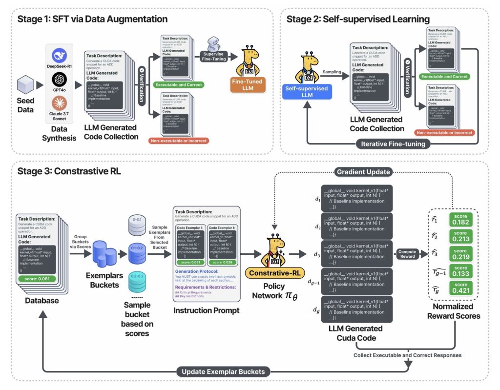
Estimated reading time: 6 minutes Table of contents The Breakthrough: Contrastive Reinforcement Learning (Contrastive-RL) How Good Is CUDA-L1? Hard Data Business Impact: Why This Matters Technical Insights: Why Contrastive-RL Wins Table: Top Techniques Discovered by CUDA-L1 Conclusion: AI Is Now Its Own Optimization Engineer AI has just unlocked triple the power from GPUs—without human intervention. DeepReinforce Team introduced a new framework called CUDA-L1 that delivers an average 3.12× speedup and up to 120× peak acceleration across 250 real-world GPU tasks. This is not mere academic promise: every result can be reproduced with open-source code, on widely used NVIDIA hardware. The Breakthrough: Contrastive Reinforcement Learning (Contrastive-RL) At the heart of CUDA-L1 lies a major leap in AI learning strategy: Contrastive Reinforcement Learning (Contrastive-RL). Unlike traditional RL, where an AI simply generates solutions, receives numerical rewards, and updates its model parameters blindly, Contrastive-RL feeds back the performance scores and prior variants directly into the next generation prompt. Performance scores and code variants are given to the AI in each optimization round. The model must then write a “Performance Analysis” in natural language—reflecting on which code was fastest, why, and what strategies led to that speedup. Each step forces complex reasoning, guiding the model to synthesize not just a new code variant but a more generalized, data-driven mental model of what makes CUDA code fast. The result? The AI discovers not just well-known optimizations, but also non-obvious tricks that even human experts often overlook—including mathematical shortcuts that entirely bypass computation, or memory strategies tuned to specific hardware quirks. The above diagram captures the three-stage training pipeline: Stage 1: The LLM is fine-tuned using validated CUDA code—collected by sampling from leading foundation models (DeepSeek-R1, GPT-4o, Claude, etc.), but retaining only correct and executable outputs. Stage 2: The model enters a self-training loop: it generates lots of CUDA code, keeps only the functional ones, and uses those to further learn. Result: rapid improvement in code correctness and coverage—all without manual labeling. Stage 3: In the Contrastive-RL phase, the system samples multiple code variants, shows each with its measured speed, and challenges the AI to debate, analyze, and outreason previous generations before producing the next round of optimizations. This reflection-and-improvement loop is the key flywheel that delivers massive speedups. How Good Is CUDA-L1? Hard Data Speedups Across the Board KernelBench—the gold-standard benchmark for GPU code generation (250 real-world PyTorch workloads)—was used to measure CUDA-L1: Model/Stage Avg. Speedup Max Speedup Median Success Rate Vanilla Llama-3.1-405B 0.23× 3.14× 0× 68/250 DeepSeek-R1 (RL-tuned) 1.41× 44.2× 1.17× 248/250 CUDA-L1 (All Stages) 3.12× 120× 1.42× 249/250 3.12× average speedup: The AI found improvements in virtually every task. 120× maximum speedup: Some computational bottlenecks and inefficient code (like diagonal matrix multiplications) were transformed with fundamentally superior solutions. Works across hardware: Codes optimized on NVIDIA A100 GPUs retained substantial gains ported to other architectures (L40, H100, RTX 3090, H20), with mean speedups from 2.37× to 3.12×, median gains consistently above 1.1× across all devices. Case Study: Discovering Hidden 64× and 120× Speedups diag(A) * B—Matrix Multiplication with Diagonal Reference (inefficient): torch.diag(A) @ B constructs a full diagonal matrix, requiring O(N²M) compute/memory. CUDA-L1 optimized: A.unsqueeze(1) * B leverages broadcasting, achieving only O(NM) complexity—resulting in a 64× speedup. Why: The AI reasoned that allocating a full diagonal was needless; this insight was unreachable via brute-force mutation, but surfaced via comparative reflection across generated solutions. 3D Transposed Convolution—120× Faster Original code: Performed full convolution, pooling, and activation—even when input or hyperparameters mathematically guaranteed all zeros. Optimized code: Used “mathematical short-circuit”—detected that given min_value=0, the output could be immediately set to zero, bypassing all computation and memory allocation. This one insight delivered orders of magnitude more speedup than hardware-level micro-optimizations. Business Impact: Why This Matters For Business Leaders Direct Cost Savings: Every 1% speedup in GPU workloads translates to 1% less cloud GPUseconds, lower energy costs, and more model throughput. Here, the AI delivered, on average, over 200% extra compute from the same hardware investment. Faster Product Cycles: Automated optimization reduces the need for CUDA experts. Teams can unlock performance gains in hours, not months, and focus on features and research velocity instead of low-level tuning. For AI Practitioners Verifiable, Open Source: All 250 optimized CUDA kernels are open-sourced. You can test the speed gains yourself across A100, H100, L40, or 3090 GPUs—no trust required. No CUDA Black Magic Required: The process doesn’t rely on secret sauce, proprietary compilers, or human-in-the-loop tuning. For AI Researchers Domain Reasoning Blueprint: Contrastive-RL offers a new approach to training AI in domains where correctness and performance—not just natural language—matter. Reward Hacking: The authors deep dive into how the AI discovered subtle exploits and “cheats” (like asynchronous stream manipulation for false speedups) and outline robust procedures to detect and prevent such behavior. Technical Insights: Why Contrastive-RL Wins Performance feedback is now in-context: Unlike vanilla RL, the AI can learn not just by trial and error, but by reasoned self-critique. Self-improvement flywheel: The reflection loop makes the model robust to reward gaming and outperforms both evolutionary approaches (fixed parameter, in-context contrastive learning) and traditional RL (blind policy gradient). Generalizes & discovers fundamental principles: The AI can combine, rank, and apply key optimization strategies like memory coalescing, thread block configuration, operation fusion, shared memory reuse, warp-level reductions, and mathematical equivalence transformations. Table: Top Techniques Discovered by CUDA-L1 Optimization Technique Typical Speedup Example Insight Memory Layout Optimization Consistent boosts Contiguous memory/storage for cache efficiency Memory Access (Coalescing, Shared) Moderate-to-high Avoids bank conflicts, maximizes bandwidth Operation Fusion High w/ pipelined ops Fused multi-op kernels reduce memory reads/writes Mathematical Short-circuiting Extremely high (10-100×) Detects when computation can be skipped entirely Thread Block/Parallel Config Moderate Adapts block sizes/shapes to hardware/task Warp-Level/Branchless Reductions Moderate Lowers divergence and sync overhead Register/Shared Memory Optimization Moderate-high Caches frequent data close to computation Async Execution, Minimal Sync Varies Overlaps I/O, enables pipelined computation Conclusion: AI Is Now Its Own Optimization Engineer With CUDA-L1, AI has become its own performance engineer, accelerating research productivity and hardware returns—without relying on rare human expertise. The

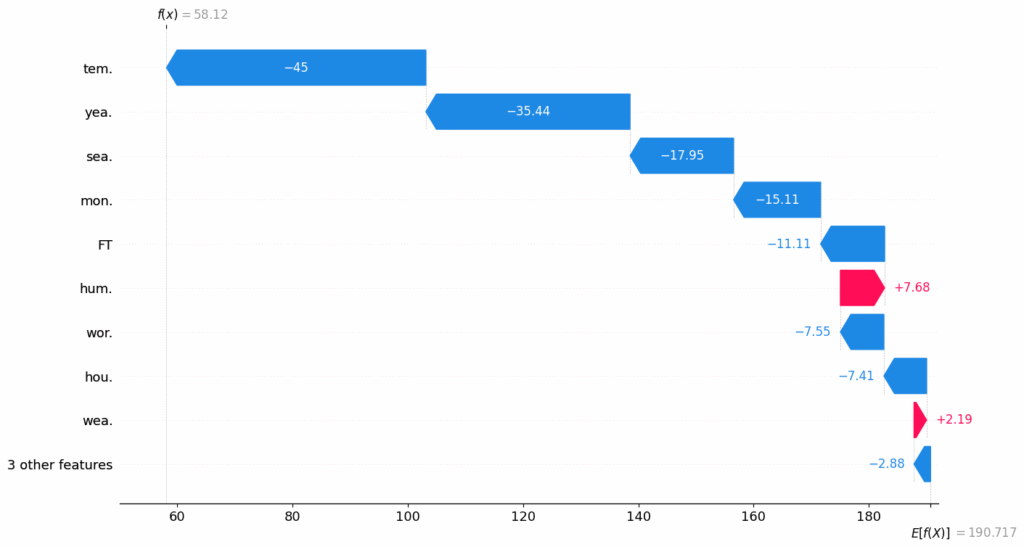
In this tutorial, we explore how to use the SHAP-IQ package to uncover and visualize feature interactions in machine learning models using Shapley Interaction Indices (SII), building on the foundation of traditional Shapley values. Shapley values are great for explaining individual feature contributions in AI models but fail to capture feature interactions. Shapley interactions go a step further by separating individual effects from interactions, offering deeper insights—like how longitude and latitude together influence house prices. In this tutorial, we’ll get started with the shapiq package to compute and explore these Shapley interactions for any model. Check out the Full Codes here Installing the dependencies Copy CodeCopiedUse a different Browser !pip install shapiq overrides scikit-learn pandas numpy Data Loading and Pre-processing In this tutorial, we’ll use the Bike Sharing dataset from OpenML. After loading the data, we’ll split it into training and testing sets to prepare it for model training and evaluation. Check out the Full Codes here Copy CodeCopiedUse a different Browser import shapiq from sklearn.ensemble import RandomForestRegressor from sklearn.metrics import mean_absolute_error, mean_squared_error, r2_score from sklearn.model_selection import train_test_split import numpy as np # Load data X, y = shapiq.load_bike_sharing(to_numpy=True) # Split into training and testing X_train, X_test, y_train, y_test = train_test_split(X, y, test_size=0.2, random_state=42) Model Training and Performance Evaluation Copy CodeCopiedUse a different Browser # Train model model = RandomForestRegressor() model.fit(X_train, y_train) # Predict y_pred = model.predict(X_test) # Evaluate mae = mean_absolute_error(y_test, y_pred) rmse = np.sqrt(mean_squared_error(y_test, y_pred)) r2 = r2_score(y_test, y_pred) print(f”R² Score: {r2:.4f}”) print(f”Mean Absolute Error: {mae:.4f}”) print(f”Root Mean Squared Error: {rmse:.4f}”) Setting up an Explainer We set up a TabularExplainer using the shapiq package to compute Shapley interaction values based on the k-SII (k-order Shapley Interaction Index) method. By specifying max_order=4, we allow the explainer to consider interactions of up to 4 features simultaneously, enabling deeper insights into how groups of features collectively impact model predictions. Check out the Full Codes here Copy CodeCopiedUse a different Browser # set up an explainer with k-SII interaction values up to order 4 explainer = shapiq.TabularExplainer( model=model, data=X, index=”k-SII”, max_order=4 ) Explaining a Local Instance We select a specific test instance (index 100) to generate local explanations. The code prints the true and predicted values for this instance, followed by a breakdown of its feature values. This helps us understand the exact inputs passed to the model and sets the context for interpreting the Shapley interaction explanations that follow. Check out the Full Codes here Copy CodeCopiedUse a different Browser from tqdm.asyncio import tqdm # create explanations for different orders feature_names = list(df[0].columns) # get the feature names n_features = len(feature_names) # select a local instance to be explained instance_id = 100 x_explain = X_test[instance_id] y_true = y_test[instance_id] y_pred = model.predict(x_explain.reshape(1, -1))[0] print(f”Instance {instance_id}, True Value: {y_true}, Predicted Value: {y_pred}”) for i, feature in enumerate(feature_names): print(f”{feature}: {x_explain[i]}”) Analyzing Interaction Values We use the explainer.explain() method to compute Shapley interaction values for a specific data instance (X[100]) with a budget of 256 model evaluations. This returns an InteractionValues object, which captures how individual features and their combinations influence the model’s output. The max_order=4 means we consider interactions involving up to 4 features. Check out the Full Codes here Copy CodeCopiedUse a different Browser interaction_values = explainer.explain(X[100], budget=256) # analyse interaction values print(interaction_values) First-Order Interaction Values To keep things simple, we compute first-order interaction values—i.e., standard Shapley values that capture only individual feature contributions (no interactions). By setting max_order=1 in the TreeExplainer, we’re saying: “Tell me how much each feature individually contributes to the prediction, without considering any interaction effects.” These values are known as standard Shapley values. For each feature, it estimates the average marginal contribution to the prediction across all possible permutations of feature inclusion. Check out the Full Codes here Copy CodeCopiedUse a different Browser feature_names = list(df[0].columns) explainer = shapiq.TreeExplainer(model=model, max_order=1, index=”SV”) si_order = explainer.explain(x=x_explain) si_order Plotting a Waterfall chart A Waterfall chart visually breaks down a model’s prediction into individual feature contributions. It starts from the baseline prediction and adds/subtracts each feature’s Shapley value to reach the final predicted output. In our case, we’ll use the output of TreeExplainer with max_order=1 (i.e., individual contributions only) to visualize the contribution of each feature. Check out the Full Codes here Copy CodeCopiedUse a different Browser si_order.plot_waterfall(feature_names=feature_names, show=True) In our case, the baseline value (i.e., the model’s expected output without any feature information) is 190.717. As we add the contributions from individual features (order-1 Shapley values), we can observe how each one pushes the prediction up or pulls it down: Features like Weather and Humidity have a positive contribution, increasing the prediction above the baseline. Features like Temperature and Year have a strong negative impact, pulling the prediction down by −35.4 and −45, respectively. Overall, the Waterfall chart helps us understand which features are driving the prediction, and in which direction—providing valuable insight into the model’s decision-making. Check out the Full Codes here. Feel free to check out our GitHub Page for Tutorials, Codes and Notebooks. Also, feel free to follow us on Twitter and don’t forget to join our 100k+ ML SubReddit and Subscribe to our Newsletter. The post How to Use the SHAP-IQ Package to Uncover and Visualize Feature Interactions in Machine Learning Models Using Shapley Interaction Indices (SII) appeared first on MarkTechPost.

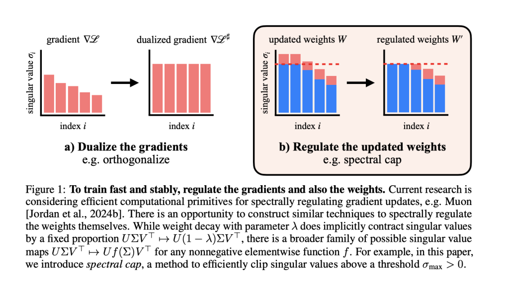
Training large-scale transformers stably has been a longstanding challenge in deep learning, particularly as models grow in size and expressivity. MIT researchers tackle a persistent problem at its root: the unstable growth of activations and loss spikes caused by unconstrained weight and activation norms. Their solution is to enforce provable Lipschitz bounds on the transformer by *spectrally regulating the weights—*with no use of activation normalization, QK norm, or logit softcapping tricks. What is a Lipschitz Bound—and Why Enforce It? A Lipschitz bound on a neural network quantifies the maximum amount by which the output can change in response to input (or weight) perturbations. Mathematically, a function fff is KKK-Lipschitz if:∥f(x1)−f(x2)∥≤K∥x1−x2∥ ∀x1,x2|f(x_1) – f(x_2)| leq K |x_1 – x_2| forall x_1, x_2∥f(x1)−f(x2)∥≤K∥x1−x2∥ ∀x1,x2 Lower Lipschitz bound ⇒ greater robustness and predictability. It is crucial for stability, adversarial robustness, privacy, and generalization, with lower bounds meaning the network is less sensitive to changes or adversarial noise. Motivation and Problem Statement Traditionally, training stable transformers at scale has involved a variety of “band-aid” stabilization tricks: Layer normalization QK normalization Logit tanh softcapping But these do not directly address the underlying spectral norm (largest singular value) growth in the weights, a root cause of exploding activations and training instability—especially in large models. The central hypothesis: If we spectrally regulate the weights themselves—beyond just the optimizer or activations—we can maintain tight control over Lipschitzness, potentially solving instability at its source. Key Innovations Weight Spectral Regulation and the Muon Optimizer Muon optimizer spectrally regularizes gradients, ensuring each gradient step does not increase the spectral norm beyond a set limit. The researchers extend regulation to the weights: After each step, they apply operations to cap the singular values of every weight matrix. Activation norms stay remarkably small as a result—rarely exceeding values compatible with fp8 precision in their GPT-2 scale transformers. Removing Stability Tricks In all experiments, no layer normalization, no QK norm, no logit tanh were used. Yet, Maximum activation entries in their GPT-2 scale transformer never exceeded ~100, while the unconstrained baseline surpassed 148,000. Table Sample (NanoGPT Experiment) Model Max Activation Layer Stability Tricks Validation Accuracy Lipschitz Bound Baseline (Speedrun) 148,480 Yes 39.4% ∞ Lipschitz Transformer 160 None 39.5% 10¹⁰²⁶⁴ Methods for Enforcing Lipschitz Constraints A variety of weight norm constraint methods were explored and compared for their ability to: Maintain high performance, Guarantee a Lipschitz bound, and Optimize the performance-Lipschitz tradeoff. Techniques Weight Decay: Standard method, but not always strict on spectral norm. Spectral Normalization: Ensures top singular value is capped, but may affect all singular values globally. Spectral Soft Cap: Novel method, smoothly and efficiently applies σ→min⁡(σmax,σ)sigma to min(sigma_{text{max}}, sigma)σ→min(σmax,σ) to all singular values in parallel (using odd polynomial approximations). This is co-designed for Muon’s high stable-rank updates for tight bounds. Spectral Hammer: Sets only the largest singular value to σmaxsigma_{text{max}}σmax, best suited for AdamW optimizer. Experimental Results and Insights Model Evaluation at Various Scales Shakespeare (Small Transformer, <2-Lipschitz): Achieves 60% validation accuracy with a provable Lipschitz bound below. Outperforms unconstrained baseline in validation loss. NanoGPT (145M Parameters): With a Lipschitz bound <10, validation accuracy: 21.2%. To match the strong unconstrained baseline (39.4% accuracy), required a large upper bound of 1026410^{264}10264. This highlights how strict Lipschitz constraints often trade off with expressivity at large scales for now. Weight Constraint Method Efficiency Muon + Spectral Cap: Leads the tradeoff frontier—lower Lipschitz constants for matched or better validation loss compared to AdamW + weight decay. Spectral soft cap and normalization (under Muon) consistently enable best frontier on the loss-Lipschitz tradeoff. Stability and Robustness Adversarial robustness increases sharply at lower Lipschitz bounds. In experiments, models with a constrained Lipschitz constant suffered much milder accuracy drop under adversarial attack compared to unconstrained baselines. Activation Magnitudes With spectral weight regulation: Maximum activations remain tiny (near-fp8 compatible), compared to the unbounded baselines, even at scale. This opens avenues for low-precision training and inference in hardware, where smaller activations reduce compute, memory, and power costs. Limitations and Open Questions Selecting the “tightest” tradeoff for weight norms, logit scaling, and attention scaling still relies on sweeps, not principle. Current upper-bounding is loose: Calculated global bounds can be astronomically large (e.g. 1026410^{264}10264), while real activation norms remain small. It’s unclear if matching unconstrained baseline performance with strictly small Lipschitz bounds is possible as scale increases—more research needed. Conclusion Spectral weight regulation—especially when paired with the Muon optimizer—can stably train large transformers with enforced Lipschitz bounds, without activation normalization or other band-aid tricks. This addresses instability at a deeper level and keeps activations in a compact, predictable range, greatly improving adversarial robustness and potentially hardware efficiency. This line of work points to new, efficient computational primitives for neural network regulation, with broad applications for privacy, safety, and low-precision AI deployment. Check out the Paper, GitHub Page and Hugging Face Project Page. Feel free to check out our GitHub Page for Tutorials, Codes and Notebooks. Also, feel free to follow us on Twitter and don’t forget to join our 100k+ ML SubReddit and Subscribe to our Newsletter. The post MIT Researchers Develop Methods to Control Transformer Sensitivity with Provable Lipschitz Bounds and Muon appeared first on MarkTechPost.