YouZum

Committee

AI, Committee, Nachrichten, Uncategorized

MoonMath AI Open-Sources a HIP Attention Kernel for AMD MI300X That Beats AITER v3 on Every Shape and Rounding Mode

MoonMath AI team has released a bf16 forward attention kernel for AMD’s MI300X GPU. It is written in HIP, not hand-written assembly. The code is open-source under the MIT license. The MoonMath.ai team reports it beats AITER v3, AMD’s own optimized kernel, on every tested shape. Bare-metal access came from HotAisle, an AMD cloud provider. Attention is the fused softmax(QKᵀ/√d)·V operation inside every transformer. The MI300X is AMD’s CDNA3 data-center GPU, with the ISA target (gfx942). This kernel runs on that hardware only. TL;DR MoonMath.ai open-sources a bf16 forward attention kernel for AMD MI300X, written in HIP, not assembly (MIT). It beats AMD’s AITER v3 on every shape and rounding mode — geomean 1.18×/1.15×/1.08×, up to 1.26×. The core trick: one-instruction asm wrappers let you pick the opcode while the compiler allocates registers. Most of the speedup is memory placement — K in LDS, V hot in L1, Q and accumulators in registers. A real SGLang PR used it to speed up Wan2.1 video diffusion by 1.23×, with no quality regression. Understanding Kernel A kernel is a small program that runs directly on the GPU’s many cores to perform one specific computation—here, the attention math—as fast as the hardware allows. The kernel computes forward attention in bf16 on MI300X only. It takes inputs in either BSHD or BHSD layout, with no transpose. Head dimension is fixed at 128. It supports any sequence length, including cross-attention. There are real limits. There is no causal mask, no GQA, and no varlen batching. Outputs are bf16, and it runs on gfx942 hardware exclusively. Numerics are tightly controlled. All three rounding modes match AITER’s per-mode rounding rule. Every finite output sits within 1 bf16 ULP of AITER. NaN and Inf handling is bit-identical, and results are deterministic. The Core Trick: One-Instruction asm Wrappers The core technique avoids a familiar dilemma. Compiler intrinsics keep code tidy but let the compiler reorder or rename operands. Raw inline assembly gives control but forces manual register and address management. MoonMath wraps exactly one instruction in a __device__ __forceinline__ function. Extended asm constraints describe the operands. The research team picks the opcode. The compiler still allocates registers and tracks data flow. Copy CodeCopiedUse a different Browser // in/out tied to the SAME VGPR → no accumulator rename, no v_mov copy. __device__ __forceinline__ void asm_mfma(bf16x4_t a, bf16x4_t b, fp32x4_t& c) { asm volatile(“v_mfma_f32_16x16x16_bf16 %0, %1, %2, %0” : “+v”(c) : “v”(a), “v”(b)); } The “+v”(c) constraint ties the accumulator input and output to the same VGPR. No copy instruction is emitted. This keeps the kernel close to ordinary HIP. It still steers the machine one instruction at a time. The Architecture: Eight Waves, Two Groups, Two Barriers A CDNA3 compute unit has four SIMD units. The textbook block is four waves. MoonMath instead runs eight waves per block, in two groups of four. The two groups run the same Q*K, softmax, O += P*V sequence. They are offset by a phase. While one group saturates the matrix core, the other runs softmax and issues loads. Then they swap, so the matrix core never idles. There are two s_barriers per iteration. One sits at the phase handoff. One sits at the iteration boundary. Per-counter waits handle the rest of the synchronization. This echoes FlashAttention-3’s matmul and softmax alternation. It does not copy FA3’s producer and consumer warp split. On CDNA3, every memory move is already asynchronous, so a dedicated producer wave is unnecessary. Where Data Lives, and Why 16×16×16 Most of the speedup comes from memory placement. K streams from HBM into LDS, double-buffered, shared by all eight waves. V stays hot in L1, read on every PV matmul. Q and accumulators live in registers. The research team picked the 16×16×16 MFMA over 32×32×8. Both shapes have identical throughput. The smaller tile accumulates into 4 fp32 elements per lane, against 16. Lower accumulator pressure leaves room for deeper prefetch and a third Q tile. Decision Choice Reason Waves per block 8 (two groups of 4) Plan the pipeline directly; share one K copy MFMA shape 16×16×16 bf16 Same throughput, lower VGPR pressure, better power efficiency K placement LDS, double-buffered, 32 KiB Shared by all 8 waves, swapped per iteration V placement L1, resident, prefetched Reread across PV, kept hot deliberately Q + accumulators VGPRs Read every iteration, never reloaded Two later wins close the gap. A third Q tile (3Q) raises data reuse per loaded K and V tile. A Flash-Decoding-style tail KV split rescues the stranded fractional round across MI300X’s 304 CUs. These wins cascade. Moving V to L1 freed the LDS that the third Q tile then fills. Benchmark Tests ran on MI300X in bf16, head dimension 128. Each shape was measured at three rounding modes. RTNE rounds to nearest even. RTNA rounds to nearest, ties away from zero. RTZ truncates toward zero. Shape (B, H, S, D) Round Ours (ms) AITER v3 (ms) vs AITER vs MAX (2, 24, 8192, 128) RTNE 3.083 3.792 1.23× 1.37× (2, 24, 16384, 128) RTNE 11.670 14.691 1.26× 1.54× (4, 16, 16384, 128) RTZ 15.055 16.183 1.07× 1.47× (2, 24, 32768, 128) RTNA 44.440 52.363 1.18× 1.57× (1, 16, 131072, 128) RTNE 232.517 269.278 1.16× 1.46× Geomeans across the sweep favor MoonMath. Versus AITER, it scores 1.18× (RTNE), 1.15× (RTNA), and 1.08× (RTZ). Versus Modular MAX, geomeans run 1.44× to 1.49×, and per-shape speedups reach 1.59×. RTZ is AITER’s own fastest mode and the tightest race. The (4, 16, 16384) RTZ shape moved from 0.95× to 1.07×. The tail KV split is what closed that final gap. Interactive Explainer Use Cases The kernel installs with pip and exposes a small API. It launches on the caller’s stream, so it overlaps inside larger pipelines. Copy CodeCopiedUse a different Browser import torch import moonmath_attention as ma # PyTorch’s ROCm build uses the “cuda” device string on AMD GPUs q = torch.randn(2, 8192, 24, 128, dtype=torch.bfloat16, device=”cuda”) k = torch.randn(2, 8192, 24, 128, dtype=torch.bfloat16, device=”cuda”) v = torch.randn(2, 8192, 24, 128, dtype=torch.bfloat16, device=”cuda”) out

MoonMath AI Open-Sources a HIP Attention Kernel for AMD MI300X That Beats AITER v3 on Every Shape and Rounding Mode Beitrag lesen »

AI, Committee, Nachrichten, Uncategorized

How to Design Python-First Interactive Dashboards with Prefab Reactive UI Components and Static HTML Export

In this tutorial, we build a Prefab application that demonstrates how to create interactive dashboards entirely in Python. We use Prefab’s component-based Python interface to design a polished operations dashboard with reactive state, charts, tables, filters, forms, tabs, alerts, metrics, and client-side actions. We generate realistic pipeline monitoring data, connect it to live UI controls, and export the final app as a static HTML dashboard that we can preview directly inside Google Colab. Through this workflow, we learn how Prefab lets us move from Python data logic to a modern React-powered user interface without having to write frontend code manually. Installing Prefab in Colab Copy CodeCopiedUse a different Browser import os import sys import base64 import subprocess from pathlib import Path from IPython.display import HTML, display, FileLink PREFAB_VERSION = “0.20.2” APP_PATH = Path(“/content/prefab_advanced_tutorial_app.py”) HTML_PATH = Path(“/content/prefab_advanced_dashboard.html”) subprocess.check_call([ sys.executable, “-m”, “pip”, “install”, “-q”, f”prefab-ui=={PREFAB_VERSION}”, ]) APP_CODE = “” We set up the Colab environment by importing the required Python utilities and defining the Prefab version, app path, and HTML export path. We install the pinned prefab-ui package so that the tutorial runs consistently without version-related issues. We also initialize an empty APP_CODE string, which we use to build the complete Prefab application step by step. Copy CodeCopiedUse a different Browser APP_CODE += r”’ Generating Synthetic Operations Data Copy CodeCopiedUse a different Browser import random from collections import Counter, defaultdict from datetime import date, timedelta from prefab_ui.actions import AppendState, OpenLink, PopState, SetState, ShowToast, ToggleState from prefab_ui.app import PrefabApp from prefab_ui.components import ( Alert, AlertDescription, AlertTitle, Badge, Button, Card, CardContent, CardDescription, CardFooter, CardHeader, CardTitle, Code, Column, DataTable, DataTableColumn, Form, Grid, H2, Input, Markdown, Mermaid, Metric, Muted, Progress, Ring, Row, Slider, Small, Switch, Tab, Tabs, Text ) from prefab_ui.components.charts import ( BarChart, ChartSeries, LineChart, PieChart, RadarChart, ScatterChart, Sparkline ) from prefab_ui.components.control_flow import Else, ForEach, If from prefab_ui.rx import EVENT, STATE random.seed(42) TODAY = date.today() DATES = [TODAY – timedelta(days=29 – i) for i in range(30)] REGIONS = [“All”, “APAC”, “EMEA”, “NA”, “LATAM”] PIPELINES = [ “Customer 360 ETL”, “Invoice OCR”, “LLM Triage”, “Risk Scoring”, “Forecast Sync”, “Warehouse Load”, ] OWNERS = [“Data Platform”, “AI Apps”, “Revenue Ops”, “Risk Engineering”] STATES = [“Completed”, “Completed”, “Completed”, “Completed”, “Late”, “Failed”] PRIORITIES = [“P0”, “P1”, “P2”, “P3”] runs = [] daily_region_rows = [] for d in DATES: for region in REGIONS[1:]: region_bias = { “APAC”: 0.96, “EMEA”: 0.94, “NA”: 0.97, “LATAM”: 0.91, }[region] volume = random.randint(32, 78) failures = 0 late = 0 total_cost = 0.0 total_latency = 0.0 total_revenue = 0.0 for i in range(volume): pipeline = random.choice(PIPELINES) owner = random.choice(OWNERS) state = random.choices( STATES, weights=[ region_bias * 10, 6, 4, 3, 1.2, max(0.2, (1 – region_bias) * 16), ], k=1, )[0] duration = max( 12, int( random.gauss(95, 35) + (20 if state == “Late” else 0) + (45 if state == “Failed” else 0) ), ) cost = round(max(0.09, random.lognormvariate(-1.15, 0.55) + duration / 1800), 2) revenue = round(random.uniform(1.2, 8.5) * (1.3 if state == “Completed” else 0.6), 2) priority = random.choices(PRIORITIES, weights=[1, 3, 7, 10], k=1)[0] if state == “Failed”: failures += 1 if state == “Late”: late += 1 total_cost += cost total_latency += duration total_revenue += revenue if d >= TODAY – timedelta(days=10) and (state in {“Failed”, “Late”} or random.random() < 0.05): runs.append({ “run_id”: f”{d.strftime(‘%m%d’)}-{region[:2]}-{len(runs)+1:04d}”, “date”: d.strftime(“%Y-%m-%d”), “pipeline”: pipeline, “owner”: owner, “region”: region, “state”: state, “priority”: priority, “duration_s”: duration, “cost_usd”: cost, “revenue_k”: revenue, “sla_gap”: round(max(0, duration – 120) / 60, 1), }) daily_region_rows.append({ “date”: d.strftime(“%b %d”), “region”: region, “runs”: volume, “failures”: failures, “late”: late, “success_rate”: round(100 * (volume – failures – late * 0.35) / volume, 1), “avg_latency”: round(total_latency / volume, 1), “cost_usd”: round(total_cost, 2), “revenue_k”: round(total_revenue, 1), }) runs = sorted( runs, key=lambda r: (r[“priority”], r[“state”] != “Failed”, -r[“duration_s”]) )[:80] def aggregate_daily(rows): by_date = defaultdict(lambda: { “date”: “”, “runs”: 0, “failures”: 0, “late”: 0, “cost_usd”: 0.0, “revenue_k”: 0.0, “latency_weighted”: 0.0, }) for r in rows: bucket = by_date[r[“date”]] bucket[“date”] = r[“date”] bucket[“runs”] += r[“runs”] bucket[“failures”] += r[“failures”] bucket[“late”] += r[“late”] bucket[“cost_usd”] += r[“cost_usd”] bucket[“revenue_k”] += r[“revenue_k”] bucket[“latency_weighted”] += r[“avg_latency”] * r[“runs”] out = [] for d in [x.strftime(“%b %d”) for x in DATES]: b = by_date[d] if b[“runs”]: b[“success_rate”] = round(100 * (b[“runs”] – b[“failures”] – b[“late”] * 0.35) / b[“runs”], 1) b[“avg_latency”] = round(b[“latency_weighted”] / b[“runs”], 1) b[“cost_usd”] = round(b[“cost_usd”], 2) b[“revenue_k”] = round(b[“revenue_k”], 1) del b[“latency_weighted”] out.append(dict(b)) return out def aggregate_regions(rows): by_region = defaultdict(lambda: { “region”: “”, “runs”: 0, “failures”: 0, “late”: 0, “cost_usd”: 0.0, “revenue_k”: 0.0, “latency_weighted”: 0.0, }) for r in rows: b = by_region[r[“region”]] b[“region”] = r[“region”] b[“runs”] += r[“runs”] b[“failures”] += r[“failures”] b[“late”] += r[“late”] b[“cost_usd”] += r[“cost_usd”] b[“revenue_k”] += r[“revenue_k”] b[“latency_weighted”] += r[“avg_latency”] * r[“runs”] out = [] for region in REGIONS[1:]: b = by_region[region] b[“success_rate”] = round(100 * (b[“runs”] – b[“failures”] – b[“late”] * 0.35) / b[“runs”], 1) b[“avg_latency”] = round(b[“latency_weighted”] / b[“runs”], 1) b[“cost_usd”] = round(b[“cost_usd”], 2) b[“revenue_k”] = round(b[“revenue_k”], 1) b[“roi”] = round(b[“revenue_k”] / max(1, b[“cost_usd”]), 1) del b[“latency_weighted”] out.append(dict(b)) return out def make_status_rows(table_rows): counts = Counter(r[“state”] for r in table_rows) return [{“state”: k, “count”: v} for k, v in counts.items()] def make_pipeline_rows(table_rows): counts = Counter(r[“pipeline”] for r in table_rows) return [{“pipeline”: k, “count”: v} for k, v in counts.most_common()] def make_kpis(region, daily_rows, table_rows): runs_count = sum(r[“runs”] for r in daily_rows) failures = sum(r[“failures”] for r in daily_rows) late = sum(r[“late”] for r in daily_rows) cost = sum(r[“cost_usd”] for r in daily_rows) revenue = sum(r[“revenue_k”] for r in daily_rows) return { “region”: region, “runs”: runs_count, “success_rate”: round(100 * (runs_count – failures – late * 0.35) / max(1, runs_count), 1), “avg_latency”: round(sum(r[“avg_latency”] * r[“runs”] for r in daily_rows) / max(1, runs_count), 1), “cost_usd”: round(cost, 2), “revenue_k”: round(revenue, 1), “roi”: round(revenue / max(1, cost), 1), “open_issues”: len(table_rows), “p0p1”: sum(1 for r in table_rows if r[“priority”] in {“P0”, “P1”}), “failure_rate”: round(100 * failures / max(1, runs_count), 2), “spark”: [r[“success_rate”] for r in daily_rows[-14:]], } DAILY_BY_REGION = {“All”: aggregate_daily(daily_region_rows)} REGION_ROWS = aggregate_regions(daily_region_rows) for region in REGIONS[1:]: DAILY_BY_REGION[region] = [r for r in daily_region_rows if r[“region”] == region] RUNS_BY_REGION = { region: [r for r in

How to Design Python-First Interactive Dashboards with Prefab Reactive UI Components and Static HTML Export Beitrag lesen »

AI, Committee, Nachrichten, Uncategorized

Inside the world’s deepest and longest subsea road tunnel

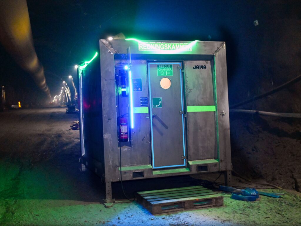
It’s cold, it’s very, very noisy, and—if I can be quite honest with you—I’m not feeling super relaxed. I’m currently around 300 meters, or 1,000 feet, beneath the North Sea, in a dark, dank cave. It smells weird. And I am increasingly aware of the pressure from millions of tons of seawater just above my head, pushing down with a force of more than 500 pounds per square inch. Picture a baby rhino standing on a postage stamp.  Only fabulous engineering is keeping me from being crushed, drowned, disappeared. My safety goggles are foggy. Just a few hundred meters away, someone is about to blow up a giant rock wall. Luckily, earlier that day I was given a full safety briefing, and I’ve got a special hard hat on. “Don’t worry—if you don’t make it, we’ll have your stuff sent back to your office,” geologist Anne-Merete Gilje tells me, straight-faced. Ah, Norwegian humor. “It’s kind of a lifestyle. You have to be a little bit crazy to work underground all the time.” Niclas Brusehed, tunnel foreman, Implenia I’m in this odd situation under the iconic fjords of Norway to visit what will soon become the world’s longest and deepest subsea road tunnel, called Rogfast (short for “Rogaland Fixed Link”). I want to understand how you make something as audacious as a 26.7-kilometer (16.6-mile) highway that sits 390 meters (1,280 feet) below the sea at its deepest point. And also—at a time when it can feel hard to get anything done, especially in the US—to reassure myself that ambitious engineering is still possible. That we can still make things.  The Norwegians already have the world’s longest subsea tunnel, the 14.4-kilometer Ryfylke, though Rogfast will dwarf it. Their expertise has attracted attention from Japan, Spain, Morocco, and even a number of US states, whose representatives were due to visit the site in May, just weeks after I went. They, too, want to know how Norway does it.  The answer: tons of explosives.  The entire endeavor feels like an obstinate refusal to give in to physics and geology. “It’s always exciting,” Niclas Brusehed, a tunnel foreman at Implenia, a Swiss firm involved in the project, tells me. “Every blast creates a new world.” There’s not just the blasting of the tunnel itself—although that is an epic project on its own—but an immense logistics challenge involving huge ventilation shafts, extreme pressure, underground roundabouts, and the complex Norwegian geology. Oh, and the water. So much water.   “This is the longest continuous blast on the sea,” says John Olaf Østerhus, assistant project manager at Implenia. “Never been done before. We can’t buy a book to see how we do this.”  All right, time to fish my phone out of my safety suit—don’t want to forget this. On another planet Arriving at the rock face where the tunnel hits seabed feels like being on the moon. It’s a huge slab of stone at the end of a long, dark, wet, wide passageway that’s lit (barely) by electric lights. Giant vehicles carting tons of rocks rumble past periodically, and we pull to the side of the road to let them by.  Rescue chambers are spread throughout the tunnel network.COURTESY OF NORWEGIAN PUBLIC ROADS ADMINISTRATION Workers clock in for 12-hour shifts, 6 a.m. until 6 p.m., deep in the bowels of the Earth where no natural light can reach. Twelve days on, 16 days off. They eat their lunch at a table in this damp cave surrounded by portacabins plastered with safety notices. “It’s kind of a lifestyle,” says Brusehed, laughing. “You have to be a little bit crazy to work underground all the time.” These crazy engineers are here to make tunnels the Norwegian way. The nation frequently uses what’s known as the drill-and-blast method instead of the tunnel-boring machines that are more typical elsewhere. This approach offers more flexibility for long, complex operations with varied rock types. Each blast adds about five to six meters to the tunnel.  Rogfast is being built inward from the ends to speed things up. The construction company Skanska is leading from the north, coming from the island of Vestre Bokn; Implenia has joined a company called Stangeland to tunnel from Randaberg in the south, which is where I am. Both teams use multiple laser scans each day to consistently measure their orientation and check that the tunnel is exactly where it should be. The two ends should meet sometime in 2029, with no more than just a few centimeters of deviation. The caves are like towering cathedrals, scattered with rubble.COURTESY OF NORWEGIAN PUBLIC ROADS ADMINISTRATION Norway has constructed more than a thousand kilometers of tunnels over the past several decades. The depth and length of these make the best efforts to date of Elon Musk’s Boring Company—a mere 2.7-kilometer tunnel in Las Vegas that is just 3.6 meters wide—look rather pathetic. The country’s spectacular setting makes such builds necessary; while Norwegians are proud of having the second-longest coastline in the world after Canada, getting up and down the west coast requires multiple ferry rides between islands, which can move extra slowly when the weather’s bad.  After it’s completed, which is scheduled to happen in 2033, Rogfast should help eliminate two ferry routes and cut the five-hour journey between the southwestern cities of Stavanger and Bergen by 40 minutes. It will funnel four lanes of traffic deep beneath the fjords of Boknafjord and Kvitsøyfjord, and at one section a relatively scant 50 meters of rock will separate the drivers speeding through the tunnel from the bottom of the North Sea. There are also, delightfully, two undersea roundabouts located 220 meters below sea level. But the first job is to contend with all that water. The never-ending battle Subsea tunneling is defined by a constant, ultimately unwinnable battle with the ocean. The sheer weight of the sea above you, and the crushing pressure, means the water will always find a way in. “It’s the volume and the pressure that’s the biggest risk,”

Inside the world’s deepest and longest subsea road tunnel Beitrag lesen »

AI, Committee, Nachrichten, Uncategorized

The Download: record-breaking subsea tunnels and flexible data centers

This is today’s edition of The Download, our weekday newsletter that provides a daily dose of what’s going on in the world of technology. Inside the world’s deepest and longest subsea road tunnel —Niall Firth I’m currently around 1,000 feet beneath the North Sea, in a dark, dank cave. It smells weird. And I’m increasingly aware of the pressure from millions of tons of seawater just above my head. I’m under the iconic fjords of Norway to visit what will soon become the world’s longest and deepest subsea road tunnel—an exceptional engineering feat that will carry drivers deep beneath the North Sea. I’m here to understand how you make a 16.6-mile highway that sits 1,280 feet below the sea at its deepest point. And also—at a time when it can feel hard to get anything done—to reassure myself that ambitious engineering is still possible. That we can still make things.  Step inside Norway’s Rogfast tunnel and see how engineers are making it happen. This story is from the next edition of our magazine, which is all about engineering. Subscribe now to get a copy when it lands on Wednesday! Want to get a data center online quickly? Give it some flex. The AI boom is putting unprecedented pressure on the electric grid. But rather than rushing to build new power plants, companies could find part of the solution right under our noses—or, more precisely, in the transmission lines under our feet and above our heads. If data centers can limit the power they draw during high-demand stretches, they won’t need to wait for big infrastructure upgrades or build their own off-grid generation. The idea of flexibility isn’t entirely foreign to grid operators. But a new generation of software could make the process faster, smarter, and more precise for the AI era. Find out how the challenge of powering AI could lead to a smarter, more flexible grid. —Amos Zeeberg The must-reads I’ve combed the internet to find you today’s most fun/important/scary/fascinating stories about technology. 1 SK Hynix has overtaken Samsung as South Korea’s most valuable companyIt’s also now the world’s most valuable memory chipmaker. (Reuters $)+  And one of the biggest beneficiaries of the global AI boom. (BBC)+ AI’s need for memory chips is set to skyrocket device prices. (WSJ $) 2 Trump says he no longer views Anthropic as a national security threat“Well, not now, but a week ago, maybe,” he told The Axios Show. (Axios)+ He praised the response of Anthropic CEO Dario Amodei. (Reuters $)+ Anthropic’s IPO outcome could depend on the midterms. (WSJ $)+ A culture war tactic against Anthropic has backfired. (MIT Technology Review) 3 SpaceX has received the lowest possible ESG ratingIndex provider MSCI gave the company a triple C. (Financial Times $)+ Russia got the same score after invading Ukraine. (Business Times)+ Elon Musk previously called ESG metrics the “Devil Incarnate.” (CNBC) 4 A Tesla on Autopilot allegedly crashed into a Texas home and killed a womanThe driver said his Tesla Model 3 was in self-driving mode. (NYT $)+ Tesla’s AI trainers don’t trust its self-driving tech. (Reuters $) 5 Polymarket reportedly paid creators to post fake betting videosClips showed them winning big on bets they would have really lost. (WSJ $)+ Polymarket bets on an Iran deal are fueling insider-trading fears. (Bloomberg $) 6 Physicists have proposed that black holes don’t existThey may be something much stranger: “gravastars.” (404 Media)+ This is the first ever photo of a black hole. (MIT Technology Review) 7 A daring space rescue mission is set to launch this weekA spacecraft will try to lift an observatory into a safer orbit. (Space)+ We’re putting more stuff into space than ever. (MIT Technology Review) 8 Nothing’s next budget phone has been cancelled due to “RAMageddon”The company said memory prices pushed costs too high. (The Verge $)+ Buying a used phone makes more sense than ever. (Wired $) 9 A viral doomsday scenario aims to pierce Europe’s AI complacencyIt envisions the US and China tearing Europe into pieces. (Guardian) 10 Scientists have invented a way to brew espresso with ultrasonic wavesNo hot water required. (Wired $) Quote of the day “Even before we start reaping the benefits of AI in our devices, we are already paying the bill.”  —Francisco Jeronimo, an analyst at IDC, tells CNBC that consumers are covering the costs of the ongoing memory shortage. One More Thing BRIAN OTIENO How mobile money supercharged Kenya’s sports betting addiction As the lorry he’d flagged down lurched through Kenya’s western highlands, Bill Kirwa’s Infinix smartphone dinged with a notification. The bet of 3,500 shillings he’d placed with mobile money—then worth approximately $35—had just turned into nearly $8,500. Kirwa, now 26, put the windfall to good use, purchasing a car that enabled him to drive for Wasili, an Uber-style ride-hailing service. But he continued gambling, and over time, his losses mounted. In just a few years, he’s effectively erased his big win.   Kirwa’s experience is hardly unique. Across Africa, the rapid spread of smartphones and mobile money has fueled an explosion in online gambling. But nowhere is the craze as acute as it is in Kenya. Find out why. —Jonathan W. Rosen We can still have nice things A place for comfort, fun, and distraction to brighten up your day. (Got any ideas? Drop me a line.) + A clever Bengal cat has seemingly learned to understand English—and talk back.+ This list of the 100 greatest bird names lovingly captures the quirks of avian taxonomy.+ Darth Vader’s weird chestplate transforms into a cassette player in these reworked Star Wars clips.+ Trace the history and evolution of heavy metal music through the interactive genres and playlists of Map of Metal.

The Download: record-breaking subsea tunnels and flexible data centers Beitrag lesen »

AI, Committee, Nachrichten, Uncategorized

Nous Research Updates Hermes Agent With a Blank Slate Mode That Pins Toolsets via platform_toolsets.cli and disabled_toolsets

Nous Research has added a Blank Slate setup mode to its open-source Hermes Agent. It inverts the usual onboarding. Instead of a fully loaded default, you start with almost nothing. Hermes Agent is the self-improving agent framework from Nous Research. It runs on your own machine. The team announced the new mode on X. Blank Slate now joins two existing options: Quick Setup and Full Setup. TL;DR Blank Slate boots an agent with everything off except provider & model, File Operations, and Terminal. Web, browser, code execution, vision, memory, delegation, cron, skills, plugins, and MCP stay disabled. It writes an explicit platform_toolsets.cli list plus agent.disabled_toolsets to pin the surface. Nothing you skipped loads later — not even after hermes update. Re-enable anything with hermes tools, hermes skills opt-in –sync, or hermes setup agent. What is Blank Slate On a fresh install, hermes setup now offers three modes. The choice sets your starting surface area. Quick Setup uses the Nous Portal. It needs no API keys and uses a free OAuth login. It sets up a model plus the Tool Gateway tools. The docs call it the recommended fast path. Full Setup is the opposite. You walk through every provider, tool, and option yourself. You bring your own keys. Blank Slate is the minimal third path. It is for building an agent from the ground up. Everything starts off except the bare minimum needed to run an agent. That minimum is three pieces: provider & model, the File Operations toolset, and the Terminal toolset. The disabled list is explicit. Off by default: web, browser, code execution, vision, memory, delegation, cron, skills, plugins, and MCP servers. Compression, checkpoints, smart routing, and memory capture are also disabled. Hermes Agent has a new Blank Slate setup mode. The default Quick/Full setup modes work great for most, but if you would rather build your agent from the ground up you can now start with just a provider, model, file operations, and terminal, then manually add in anything else. pic.twitter.com/EiFm7tW3Ws — Nous Research (@NousResearch) June 20, 2026 The Two Paths After the Baseline Blank Slate does not stop at the baseline. After the minimal baseline is applied, you choose one of two paths. The first path keeps everything disabled. You finish now with the minimal agent. You get file and terminal access, and nothing else. The second path walks through all configurations. You opt in to tools, skills, plugins, MCP, and messaging. You enable only what each workflow needs. Pick Blank Slate when you want a minimal, fully-controlled agent. The point is to enable exactly what you need and no more. Why the Config Format Matters Blank Slate does not just toggle features at runtime. It writes the decision to disk. The mode writes an explicit platform_toolsets.cli list. It also writes agent.disabled_toolsets. Together, these two keys pin your agent’s surface. The effect is durable. Nothing you did not choose ever loads. That holds even after hermes update. An update cannot silently re-enable a toolset you left off. Hermes also separates secrets from settings. Tokens live in ~/.hermes/.env. Non-secret settings live in ~/.hermes/config.yaml. The CLI routes each value to the correct file. Setup Modes Compared Mode Enabled by default Keys / auth Best for Quick Setup (Nous Portal) Model + Tool Gateway tools Free OAuth, no API keys Fastest first run Full Setup Every tool and option you pick Bring your own keys Hand-tuned, full control Blank Slate Provider & model, File Operations, Terminal Provider auth only Minimal, fully-controlled setups Use Cases With Examples Three situations fit Blank Slate well: A security-sensitive deployment is the first. You want an agent with no web and no browser. Blank Slate ships file and terminal access only. Nothing reaches the network unless you add it. A reproducible team setup is the second. You pin one known toolset across every machine. Updates will not drift the configuration. New tools never appear without an explicit opt-in. A teaching or audit environment is the third. You start minimal and add one toolset at a time. Each capability becomes a deliberate choice. Here is a minimal flow. Install, run setup, choose Blank Slate, then finish now. Copy CodeCopiedUse a different Browser curl -fsSL https://hermes-agent.nousresearch.com/install.sh | bash source ~/.bashrc # or source ~/.zshrc hermes setup # choose Blank Slate, then “finish now” hermes # file + terminal only Later, add one capability when a task needs it. Copy CodeCopiedUse a different Browser hermes tools # re-enable a toolset, e.g. web hermes skills opt-in –sync # seed skills on demand hermes setup agent # tune compression, routing, memory A Note for Local Setups Hermes Agent requires a model with at least 64,000 tokens of context. Smaller windows are rejected at startup. Most hosted models meet this easily. Local models need an explicit context size of 64K. For example, use –ctx-size 65536 for llama.cpp. A minimal Blank Slate agent on a local model still has to clear this floor. Interactive Explainer Check out the Technical details. Also, feel free to follow us on Twitter and don’t forget to join our 150k+ML SubReddit and Subscribe to our Newsletter. Wait! are you on telegram? now you can join us on telegram as well. Need to partner with us for promoting your GitHub Repo OR Hugging Face Page OR Product Release OR Webinar etc.? Connect with us The post Nous Research Updates Hermes Agent With a Blank Slate Mode That Pins Toolsets via platform_toolsets.cli and disabled_toolsets appeared first on MarkTechPost.

Nous Research Updates Hermes Agent With a Blank Slate Mode That Pins Toolsets via platform_toolsets.cli and disabled_toolsets Beitrag lesen »

AI, Committee, Nachrichten, Uncategorized

Crawlee for Python: Build a Web Crawling Pipeline with Robots Handling, Link Graphs, and RAG Chunk Export

In this tutorial, we build a full Crawlee-for-Python workflow that covers environment setup, local website generation, static crawling, dynamic crawling, structured extraction, and downstream data processing. We begin by configuring a compatible Crawlee runtime with pinned Pydantic support, Playwright browser installation, persistent storage directories, and Colab-safe execution handling. We then generate a realistic local demo website containing product pages, documentation pages, blog content, internal links, robots.txt rules, JSON-LD metadata, and JavaScript-rendered catalog items. Using BeautifulSoupCrawler, we perform fast recursive HTML crawling and extract page titles, metadata, text previews, outgoing links, product attributes, documentation headings, code blocks, and blog tags. With ParselCrawler, we run precise CSS- and XPath-based extraction on product detail pages. With PlaywrightCrawler, we render JavaScript content in a headless Chromium browser, wait for dynamic DOM elements to appear, extract client-side data, and capture full-page screenshots. Setting Up the Crawlee Python Runtime and Helpers Copy CodeCopiedUse a different Browser import os import sys import re import csv import json import time import math import shutil import socket import hashlib import asyncio import textwrap import subprocess import threading from pathlib import Path from functools import partial from http.server import ThreadingHTTPServer, SimpleHTTPRequestHandler from importlib.metadata import version, PackageNotFoundError SETUP_SENTINEL = “/content/.crawlee_python_tutorial_setup_done_v2″ def sh(command, check=True, quiet=False): print(f”n$ {command}”) result = subprocess.run( command, shell=True, text=True, stdout=subprocess.PIPE, stderr=subprocess.STDOUT, ) if not quiet and result.stdout: print(result.stdout[-5000:]) if check and result.returncode != 0: raise RuntimeError(f”Command failed with exit code {result.returncode}: {command}”) return result.returncode == 0 def package_version(package_name): try: return version(package_name) except PackageNotFoundError: return None def is_good_pydantic_version(v): if not v: return False m = re.match(r”^(d+).(d+)”, v) if not m: return False major, minor = int(m.group(1)), int(m.group(2)) return major == 2 and minor == 11 current_crawlee = package_version(“crawlee”) current_pydantic = package_version(“pydantic”) needs_setup = ( not os.path.exists(SETUP_SENTINEL) or current_crawlee is None or not is_good_pydantic_version(current_pydantic) ) if needs_setup: print(“PHASE 1: Installing compatible Crawlee + Pydantic + Playwright dependencies.”) print(“After this finishes, Colab will restart automatically. Then run this same cell again.”) sh(f'{sys.executable} -m pip uninstall -y crawlee pydantic pydantic-core’, check=False) sh( f'{sys.executable} -m pip install -q -U ‘ f'”pydantic>=2.11,<2.12″ ‘ f'”crawlee[all]” ‘ f’pandas matplotlib networkx nest_asyncio beautifulsoup4 parsel’ ) sh(f'{sys.executable} -m playwright install –with-deps chromium’, check=False) Path(SETUP_SENTINEL).write_text(“done”, encoding=”utf-8″) print(“nInstalled versions:”) sh(f'{sys.executable} -m pip show crawlee pydantic pydantic-core’, check=False) try: import google.colab print(“nRestarting Colab runtime now. After it reconnects, run this same cell again.”) os.kill(os.getpid(), 9) except Exception: raise SystemExit(“Setup complete. Restart the runtime/kernel manually, then run this cell again.”) print(“PHASE 2: Dependencies are ready. Running the Crawlee tutorial.”) import pandas as pd import matplotlib.pyplot as plt import networkx as nx import nest_asyncio nest_asyncio.apply() TUTORIAL_ROOT = Path(“/content/crawlee_python_advanced_tutorial”) SITE_DIR = TUTORIAL_ROOT / “demo_site” OUTPUT_DIR = TUTORIAL_ROOT / “outputs” STORAGE_DIR = TUTORIAL_ROOT / “crawlee_storage” SCREENSHOT_DIR = OUTPUT_DIR / “screenshots” for path in [SITE_DIR, OUTPUT_DIR, STORAGE_DIR]: if path.exists(): shutil.rmtree(path) for path in [SITE_DIR, OUTPUT_DIR, STORAGE_DIR, SCREENSHOT_DIR]: path.mkdir(parents=True, exist_ok=True) os.environ[“CRAWLEE_STORAGE_DIR”] = str(STORAGE_DIR) os.environ[“CRAWLEE_LOG_LEVEL”] = “INFO” os.environ[“CRAWLEE_PURGE_ON_START”] = “true” from crawlee import Glob, ConcurrencySettings from crawlee.crawlers import ( BeautifulSoupCrawler, BeautifulSoupCrawlingContext, ParselCrawler, ParselCrawlingContext, PlaywrightCrawler, PlaywrightCrawlingContext, ) try: import crawlee print(“Crawlee version:”, crawlee.__version__) except Exception: print(“Crawlee imported successfully.”) print(“Pydantic version:”, package_version(“pydantic”)) def safe_slug(value): value = re.sub(r”[^a-zA-Z0-9]+”, “-“, str(value)).strip(“-“).lower() return value or “item” def money_to_float(value): if value is None: return None cleaned = re.sub(r”[^0-9.]”, “”, str(value)) return float(cleaned) if cleaned else None def normalize_text(value, max_len=None): value = re.sub(r”s+”, ” “, value or “”).strip() return value[:max_len] if max_len else value def write_file(path, content): path = Path(path) path.parent.mkdir(parents=True, exist_ok=True) path.write_text(textwrap.dedent(content).strip() + “n”, encoding=”utf-8″) We begin by preparing the complete Colab runtime for the Crawlee tutorial. We install compatible versions of Crawlee, Pydantic, Playwright, and the required analysis libraries, and handle the automatic restart required after setup. We then configure storage folders, environment variables, crawler imports, and helper functions to ensure the rest of the workflow runs smoothly. Generating the Demo Website and Product Catalog Copy CodeCopiedUse a different Browser PRODUCTS = [ { “sku”: “CRW-101”, “name”: “Crawler Reliability Kit”, “category”: “automation”, “price”: 149.0, “rating”: 4.8, “stock”: 18, “features”: [“retry policy”, “queue replay”, “structured logs”], “related”: [“CRW-202”, “CRW-303”], }, { “sku”: “CRW-202”, “name”: “Playwright Rendering Pack”, “category”: “browser”, “price”: 249.0, “rating”: 4.7, “stock”: 9, “features”: [“headless chromium”, “screenshots”, “dynamic DOM extraction”], “related”: [“CRW-101”, “CRW-404”], }, { “sku”: “CRW-303”, “name”: “RAG Extraction Bundle”, “category”: “ai-data”, “price”: 199.0, “rating”: 4.9, “stock”: 13, “features”: [“clean text chunks”, “metadata capture”, “JSONL export”], “related”: [“CRW-101”, “CRW-505”], }, { “sku”: “CRW-404”, “name”: “Anti-Fragile Session Toolkit”, “category”: “resilience”, “price”: 299.0, “rating”: 4.6, “stock”: 5, “features”: [“session rotation”, “state recovery”, “graceful failures”], “related”: [“CRW-202”, “CRW-505”], }, { “sku”: “CRW-505”, “name”: “Data Export Control Plane”, “category”: “storage”, “price”: 179.0, “rating”: 4.5, “stock”: 21, “features”: [“datasets”, “key-value store”, “CSV and JSON export”], “related”: [“CRW-303”, “CRW-404″], }, ] def layout(title, body, extra_head=””, extra_script=””): css = “”” <style> body { font-family: Inter, system-ui, -apple-system, BlinkMacSystemFont, “Segoe UI”, sans-serif; margin: 0; background: #f7f7fb; color: #1f2430; } header { background: #202638; color: white; padding: 28px 40px; } nav a { color: #dbe7ff; margin-right: 18px; text-decoration: none; font-weight: 600; } main { max-width: 1050px; margin: 0 auto; padding: 32px; } .grid { display: grid; grid-template-columns: repeat(auto-fit, minmax(230px, 1fr)); gap: 18px; } .card, article, .panel { background: white; border: 1px solid #e5e7ef; border-radius: 16px; padding: 20px; box-shadow: 0 8px 25px rgba(20, 30, 60, 0.05); } .price { font-size: 1.3rem; font-weight: 800; } .tag { display: inline-block; background: #edf2ff; border: 1px solid #d6e0ff; border-radius: 999px; padding: 4px 10px; margin: 3px; font-size: 0.82rem; } .stock-low { color: #b42318; font-weight: 700; } .stock-ok { color: #067647; font-weight: 700; } code, pre { background: #111827; color: #d1fae5; border-radius: 10px; } pre { padding: 16px; overflow-x: auto; } footer { padding: 30px 40px; color: #606779; } </style> “”” return f””” <!doctype html> <html lang=”en”> <head> <meta charset=”utf-8″> <meta name=”viewport” content=”width=device-width, initial-scale=1″> <meta name=”description” content=”{title} page for a Crawlee Python tutorial demo website.”> <title>{title}</title> {css} {extra_head} </head> <body> <header> <h1>{title}</h1> <nav> <a href=”/index.html”>Home</a> <a href=”/products/product-crw-101.html”>Products</a> <a href=”/docs/getting-started.html”>Docs</a> <a href=”/blog/crawling-at-scale.html”>Blog</a> <a href=”/dynamic.html”>Dynamic JS Page</a> <a href=”/admin/hidden.html”>Admin</a> </nav> </header> <main>{body}</main> <footer>Local demo website generated for Crawlee Python advanced tutorial.</footer> {extra_script} </body> </html> “”” def build_demo_site(): write_file( SITE_DIR / “robots.txt”, “”” User-agent: * Disallow: /admin/ Allow: /

Crawlee for Python: Build a Web Crawling Pipeline with Robots Handling, Link Graphs, and RAG Chunk Export Beitrag lesen »

AI, Committee, Nachrichten, Uncategorized

VibeThinker-3B: A 3B Dense Reasoning Model Built on Qwen2.5-Coder-3B With the Spectrum-to-Signal Post-Training Pipeline

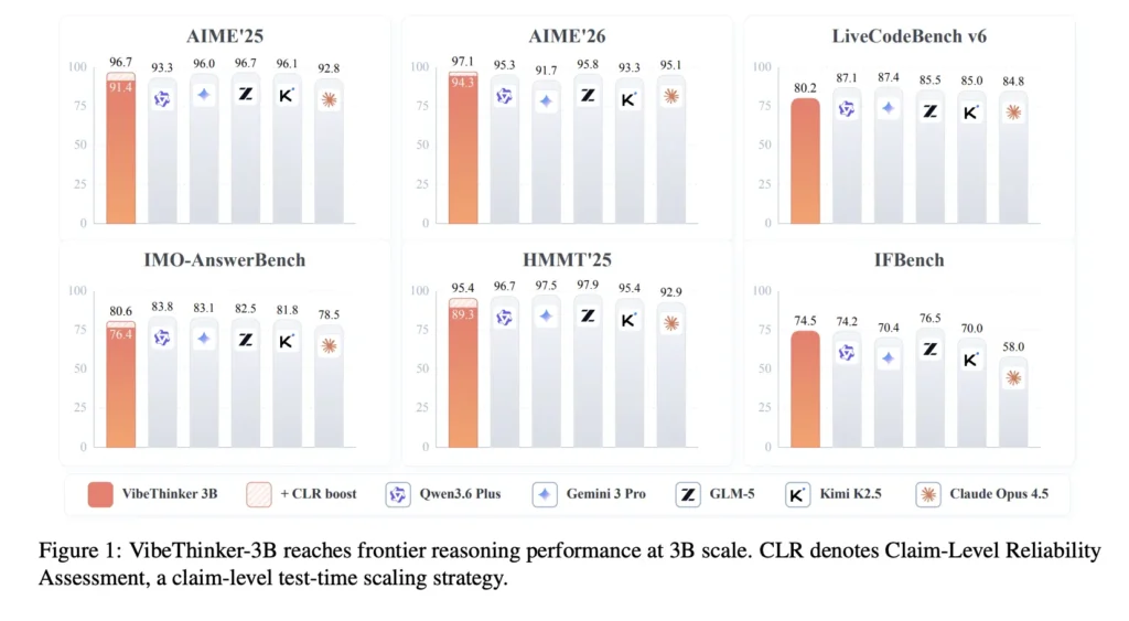
While recent breakthroughs in AI reasoning have largely been driven by massive scale, pouring in billions of parameters to cross complex cognitive thresholds—VibeThinker-3B is charting a completely different path. Created by researchers from Sina Weibo Inc (China), this 3-billion-parameter model proves that efficiency can punch far above its weight class. Released under an open-source MIT license, VibeThinker-3B matches the performance of models hundreds of times its size on verifiable tasks like mathematics, coding, and STEM disciplines. What is VibeThinker-3B VibeThinker-3B is a compact dense model built on the Qwen2.5-Coder-3B base. It is post-trained, not pretrained from scratch. The research team applies supervised fine-tuning, reinforcement learning, and self-distillation on top. The training framework continues the Spectrum-to-Signal Principle (SSP) from the earlier VibeThinker-1.5B. SFT (Supervised Fine-Tuning) builds a broad space of valid reasoning paths, the ‘Spectrum.’ RL then amplifies the correct paths, the ‘Signal.’ The model targets one job: reasoning where a verifier can confirm the answer. The research team recommends larger general models for open-domain knowledge tasks. VibeThinker-3B is a specialist by design. It runs on standard stacks. The model weights require transformers>=4.54.0. For faster inference it recommends vLLM==0.10.1 or SGLang>=0.4.9.post6. The BF16 weights are roughly 6 GB, small enough for a single GPU. https://arxiv.org/pdf/2606.16140v1 Benchmark On AIME26, VibeThinker-3B scores 94.3. According to the research paper, this is comparable to DeepSeek V3.2 (671B) and Kimi K2.5 (1T). On LiveCodeBench v6, it reaches 80.2 Pass@1. On OJBench, another code benchmark, it scores 38.6, below the largest models. On HMMT25 it scores 89.3, and on BruMO25 it reaches 93.8. On IMO-AnswerBench, a 400-problem IMO-level set, it scores 76.4. The table below compares it against much larger reasoning models. The ‘+CLR’ row uses test-time scaling. It stands for Claim-Level Reliability Assessment Model Params AIME26 HMMT25 IMO-Ans LCBv6 GPQA-D VibeThinker-3B 3B 94.3 89.3 76.4 80.2 70.2 VibeThinker-3B +CLR 3B 97.1 95.4 80.6 — 72.9 GPT-OSS (high) 120B 93.2 90.0 75.6 81.9 80.1 DeepSeek V3.2 671B 94.2 90.2 78.3 80.8 82.4 GLM-5 744B 95.8 97.9 82.5 85.5 86.0 Kimi K2.5 1T 93.3 95.4 81.8 85.0 87.6 Source: VibeThinker-3B Technical Report, Table 2. GPQA-D is GPQA-Diamond. The pattern is consistent. On verifiable math and code, the 3B model sits near the top cluster. On GPQA-Diamond, a knowledge-heavy benchmark, the gap to large models stays visible. The research team also ran an out-of-distribution coding test. It used recent LeetCode weekly and biweekly contests, from Apr 25 to May 31, 2026. The model passed 123 of 128 first-attempt Python submissions. That is a 96.1% acceptance rate on unseen problems. Inside the Spectrum-to-Signal Pipeline The post-training pipeline runs in four stages. Each one targets a different weakness of small reasoning models. First comes curriculum-based two-stage SFT. Stage 1 covers math, code, STEM, dialogue, and instruction following broadly. Stage 2 shifts to harder, longer-horizon samples filtered by reasoning length and difficulty. Diversity-Exploring Distillation preserves multiple valid solution paths through both stages. Second comes multi-domain Reasoning RL. The research team reuses MaxEnt-Guided Policy Optimization (MGPO). MGPO weights prompts near the model’s current capability boundary, where correct and incorrect rollouts coexist. Training runs sequentially across Math, Code, and STEM. A notable detail: VibeThinker-3B drops progressive context expansion. The research team found high-truncation warm-up hurt long reasoning at this scale. So RL uses a single 64K long-context window throughout. Math RL adds a Long2Short stage. It redistributes reward among correct trajectories by length. Shorter correct answers get higher reward, longer ones lower, with the group mean unchanged. The goal is fewer redundant tokens without losing accuracy. Third, Offline Self-Distillation merges the RL checkpoints back into one student model. Fourth, Instruct RL improves instruction adherence. That stage explains the 93.4 IFEval and 74.5 IFBench scores. Both show reasoning tuning did not break controllability. CLR: Scaling at Test Time, Not Parameter Count Claim-Level Reliability Assessment (CLR) is the report’s test-time scaling method. It runs on answer-verifiable tasks and adds no parameters. The procedure has two steps. The model first generates K = 32 trajectories per problem. From each, it extracts M = 5 decision-relevant claims plus a final answer. The model then acts as its own verifier. It validates or falsifies each claim, producing binary verdicts. CLR maps these into a nonlinear trajectory reliability score, where one weak claim sharply lowers the weight. Answers are clustered by equivalence, and the highest reliability-weighted answer wins. The full flow runs 8 times, and the averaged Pass@1 is reported. CLR lifts AIME26 to 97.1 and BruMO25 to 99.2. The interactive demo below lets you flip claims and watch the score collapse. It also lets you switch benchmarks and compare against larger models. Use Cases With Examples The research team frames VibeThinker-3B as a specialist, so use cases follow the verifiable-reasoning boundary. Competitive math tutoring: It solves AIME and HMMT-style problems with full chains of reasoning. A study tool could generate worked solutions and self-check answers locally. Algorithmic coding help: The 96.1% LeetCode acceptance rate suggests strong one-shot Python generation. An IDE assistant could draft contest-style solutions and run hidden tests. Cost-sensitive RL or agent backends: A 3B model is cheap to serve at scale. Teams running many verifiable subtasks could route them here instead of a 600B+ model. On-device reasoning. BF16 weights fit one consumer GPU. Edge or offline deployments gain a reasoning engine without cloud calls. Running It: Quick Start Serving with vLLM exposes an OpenAI-compatible endpoint: Copy CodeCopiedUse a different Browser pip install vllm vllm serve “WeiboAI/VibeThinker-3B” curl -X POST “http://localhost:8000/v1/chat/completions” -H “Content-Type: application/json” –data ‘{ “model”: “WeiboAI/VibeThinker-3B”, “messages”: [{“role”:”user”,”content”:”Prove there are infinitely many primes.”}], “temperature”: 1.0, “top_p”: 0.95 }’ Direct Transformers usage mirrors the official card: Copy CodeCopiedUse a different Browser from transformers import AutoModelForCausalLM, AutoTokenizer tok = AutoTokenizer.from_pretrained(“WeiboAI/VibeThinker-3B”, trust_remote_code=True) model = AutoModelForCausalLM.from_pretrained( “WeiboAI/VibeThinker-3B”, torch_dtype=”bfloat16″, device_map=”auto”) msgs = [{“role”: “user”, “content”: “Your prompt”}] text = tok.apply_chat_template(msgs, tokenize=False, add_generation_prompt=True) inputs = tok([text], return_tensors=”pt”).to(model.device) out = model.generate(**inputs, max_new_tokens=102400, do_sample=True, temperature=1.0, top_p=0.95) print(tok.decode(out[0][inputs.input_ids.shape[-1]:], skip_special_tokens=True)) The high max_new_tokens matters. The model produces long reasoning traces, so short caps can truncate answers. Key Takeaways VibeThinker-3B is a 3B dense model,

VibeThinker-3B: A 3B Dense Reasoning Model Built on Qwen2.5-Coder-3B With the Spectrum-to-Signal Post-Training Pipeline Beitrag lesen »

AI, Committee, Nachrichten, Uncategorized

NVIDIA AI Introduce SpatialClaw: A Training-Free Agent That Treats Code as the Action Interface for Spatial Reasoning

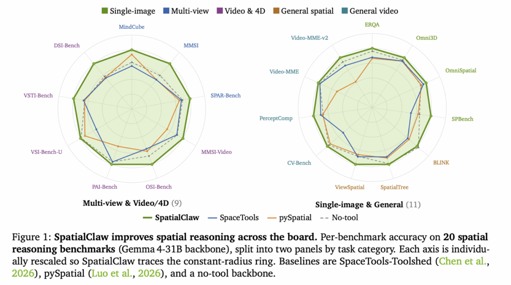
NVIDIA Research has released SpatialClaw, a training-free framework for spatial reasoning. It targets a persistent weakness in vision-language models (VLMs). These models still struggle to judge where objects are, how they relate, and how they move in 3D. SpatialClaw does not retrain the model. Instead, it changes the action interface the agent uses to call perception tools. The research team argues the interface is the bottleneck. Their solution is to treat code as the action interface. Across 20 benchmarks, SpatialClaw reaches 59.9% average accuracy. It outperforms the recent spatial agent SpaceTools by 11.2 points. What is SpatialClaw SpatialClaw is an agent loop wrapped around a stateful Python kernel. The kernel is pre-loaded with input frames and a set of primitives. Perception tools are plain Python callables. Their outputs, including masks, depth maps, camera geometry, and trajectories, are ordinary Python variables. The kernel exposes six public entry points. InputImages holds the sampled frames. Metadata carries frame rate, duration, and frame indices. tools exposes perception and geometry primitives. show() embeds an image into the agent’s next context. vlm dispatches queries to a separate VLM session. ReturnAnswer() submits the final answer. Two perception tools are central. tools.Reconstruct wraps Depth Anything 3 and returns per-frame depth, camera intrinsics, extrinsics, and dense point maps. tools.SAM3 wraps SAM 3 and produces image or video masks from text, point, or box prompts. The framework adds lightweight utilities: tools.Geometry, tools.Mask, tools.Time, tools.Graph, and tools.Draw. It is training-free. The same system prompt, tool set, and hyperparameters run across every benchmark and backbone. https://spatialclaw.github.io/static/pdfs/spatialclaw.pdf Why the Action Interface Matters The research team studied three action interfaces on the same question. Consider measuring the closest distance between a heater and a door. Single-pass code writes one complete program and runs it once. It commits to a full strategy before seeing any intermediate mask or depth map. A wrong assumption then propagates straight to the answer. Structured tool-call invokes named tools through a fixed JSON schema. It cannot freely combine outputs with NumPy or SciPy to express test-time computations. The closest-point operation has no pre-registered tool, so the result is wrong. SpatialClaw composes tools in code, inspects results, then revises. It first computes a centroid distance, then notices the centroid uses a median. The agent switches to scipy.spatial.KDTree to find the true closest point. It submits 0.9439 m against a 0.9 m ground truth. Benchmark SpatialClaw was tested on 20 benchmarks across five categories. These span single-image, multi-view, general, video and 4D, and general video understanding. It improves over the no-tool baseline on all six backbones tested. Backbones range from 26B to 397B parameters across the Qwen3.5/3.6 and Gemma4 families. A controlled comparison isolates the interface. All three variants share the same toolset and prompt. Only the action interface differs. Action interface Avg. (20 bench.) Δ vs no-tool No-tool baseline 53.4 – Single-pass code 55.2 +1.8 Structured tool-call 56.7 +3.3 SpatialClaw (code as action) 59.9 +6.5 Gemma4-31B backbone, 20-benchmark average. Against prior spatial agents on the same Gemma4-31B backbone, the gap widens. Method Interface Avg. Δ vs SpatialClaw VADAR Single-pass 40.5* −19.4 pySpatial Single-pass 47.8 −12.1 SpaceTools-Toolshed Structured tool-call 48.7 −11.2 SpatialClaw Code as action 59.9 best VADAR does not support video or multi-image inputs; only single-image benchmarks are averaged. The largest gains land on dynamic tasks. On Gemma4-31B, DSI-Bench rose +17.6 points and MindCube rose +15.3 points. These categories need chained geometric computation across frames and viewpoints. An LLM-as-judge attribution explains the wins over structured tool-call. Code composition accounts for 52.2% of them. Control flow accounts for 19.5%, and the remaining 28.3% are interface-neutral. Inside the Five-Stage Loop Each sample runs a five-stage loop: planning, code generation, code execution, feedback assembly, and answer submission. A planner drafts a strategy without seeing the images. The main agent then writes one Python cell per step. A static AST checker rejects unsafe code before execution. The loop repeats until ReturnAnswer() is called or 30 steps pass. The official repo runs on a LangGraph workflow and a persistent Jupyter kernel. Backbones serve through vLLM. Perception runs behind a FastAPI GPU service. A single quickstart runs one benchmark on one machine: Copy CodeCopiedUse a different Browser git clone –recursive https://github.com/NVlabs/SpatialClaw.git cd SpatialClaw bash spatial_agent/scripts/setup.sh cp .env.example .env # add API keys, or self-host vLLM python -m spatial_agent.entrypoints.run –dataset spatial_agent/config/dataset/erqa.json –model spatial_agent/config/model/gemini-3-pro.json –concurrency 4 A representative agent cell composes perception with geometry, then revises: Copy CodeCopiedUse a different Browser # Reconstruct the scene, then segment both objects in one video pass recon = tools.Reconstruct.Reconstruct(InputImages) seg = tools.SAM3.segment_video_by_text([“radiator heater”, “door”]) show(seg.visualize(1)) # inspect the masks first # Closest-point distance via KD-tree, not centroids pts_h = seg.get_masked_points(recon, frame=1, object=0) # object 0 = heater pts_d = seg.get_masked_points(recon, frame=2, object=1) # object 1 = door dists, _ = scipy.spatial.KDTree(pts_d).query(pts_h, k=1) ReturnAnswer(float(dists.min())) The agent picks primitives from the question itself. Distance questions invoke KD-tree search and vector norms. Direction questions rely on dot products. No category-specific routing was applied. Use Cases The design fits problems that need step-by-step geometric reasoning. Concrete examples include: Robotics and embodied agents that measure metric distances between objects before acting. Multi-view inspection, where an object’s facing direction is recovered from several camera angles. Video and 4D analysis that tracks object or camera motion across frames. Indoor scene question answering, such as “where is the door relative to the sink?” Because it is training-free, teams can extend a deployed VLM without new data or fine-tuning. Interactive Explainer Back</button> <button class="”c" primary” id="”sc-next”">Run next step </button> <button class="”c”" id="”sc-reset”">Reset</button> <span class="”prog”" id="”sc-prog”"></span> </div> <div class="”foot”"> <span>Faithful to the paper’s walkthrough · interface logic is illustrative</span> <span>Built for <b>Marktechpost</b> · verified Jun 2026</span> </div> </div> <script> (function(){ var root=document.getElementById(‘sc-root’); if(!root)return; var $=function(s){return root.querySelector(s)}; // — step data, faithful to Figure 2 of the SpatialClaw paper — var DATA={ single:{ label:”single-pass · no persistence”, stateNote:”No intermediate state. One complete program is committed before any execution feedback is seen.”, vars:[], steps:[{ think:”Write one complete program now, before seeing any mask, depth map, or error.”, code:'<span class="”cm”"># commit the full analysis

NVIDIA AI Introduce SpatialClaw: A Training-Free Agent That Treats Code as the Action Interface for Spatial Reasoning Beitrag lesen »

AI, Committee, Nachrichten, Uncategorized

Yandex Open-Sources YaFF: A Zero-Copy Wire Format for Protobuf With Near-Struct Read Speed

TLDR YaFF is Yandex’s open-source zero-copy wire format for Protobuf — Apache 2.0, currently C++, v0.1.0. The .proto file stays the source of truth; only the physical memory layout changes. On Yandex’s benchmarks, the Flat Layout reads hot data ~3.8× faster than FlatBuffers, within 1.2× of a raw C++ struct. Four layouts — Fixed, Flat, Sparse, Dynamic — trade read speed for schema flexibility; Dynamic is the default. YaFF runs in its advertising recommendation system, where it reports 10–20% CPU savings at production scale.  Adoption is incremental: drop it into one hot path, with two-way Protobuf conversion at the edges. Yandex has open-sourced YaFF (Yet another Flat Format) under Apache 2.0. It is a high-performance C++ serialization library. YaFF provides a zero-copy wire format for the Protobuf ecosystem. Your .proto file stays the single source of truth. The format only changes how data sits in memory. It concentrates on server-side runtimes. What is YaFF  YaFF is not a replacement for Protobuf. It is an alternative wire format for Protobuf messages. The same .proto schema generates a proto-like C++ API. Reads need no parsing step, so fields come straight from the buffer. Less performance-sensitive code can still parse the wire format back into Protobuf messages. That two-way conversion is what makes module-by-module adoption realistic. You introduce YaFF in one hot path and leave the rest on Protobuf. The Problem it Targets Protobuf parsing can consume double-digit percentages of CPU in high-load backends. At scale, that maps to thousands of physical cores. The common  zero-copy option  is FlatBuffers, also from Google. But FlatBuffers is not a Protobuf drop-in and requires maintaining a separate schema and conversion layer. semantically incompatible with Protobuf. Migrating means duplicated schemas, different schema-evolution rules , and hand-written field converters. Many teams conclude the cost is not worth it. YaFF aims at that gap: zero-copy reads with Protobuf semantics preserved. How the Layouts Work A layout decides how a message is stored in the buffer. It changes only the physical representation, leaving the schema and generated interfaces unchanged. YaFF ships four layouts. Fixed is a plain packed struct with no header and a frozen schema. Flat adds a two-byte header and supports schema evolution. Sparse addresses fields through a meta table, fitting sparse schemas. Dynamic is the default and selects Flat or Sparse at runtime. It uses Flat while the schema permits, then switches to Sparse when evolution breaks flat alignment. Layout Read access Per-message overhead Schema evolution Best for Fixed 1 read, 0 branches 0 bytes Frozen Small inlined primitives Flat 2 reads, 1 branch 2 bytes Restricted (type preservation) Dense, hot data Sparse 4 reads, 2 branches 6 bytes Unrestricted Sparse schemas, free evolution Dynamic (default) Flat or Sparse at runtime 2 or 6 bytes Unrestricted General application logic Benchmark Yandex ships a reproducible benchmark suite, built with google/benchmark in a Release build. The numbers below are median nanoseconds per read on an AMD EPYC 7713 with Clang 20.1.8. Lower is faster. In the hot hierarchical case, the Flat Layout reads in 9.79 ns. FlatBuffers needs 37.30 ns, and Protobuf needs 219.35 ns. The raw C++ struct baseline is 8.14 ns. So the Flat Layout reads about 3.8× faster than FlatBuffers here, and about 22× faster than Protobuf. It stays within 1.2× of the raw struct. Format Read time (ns) Slowdown vs raw struct Raw C++ struct 8.14 1.0× YaFF Flat Layout 9.79 1.2× YaFF Sparse Layout 21.23 2.6× FlatBuffers 37.30 4.6× Protobuf 219.35 26.9× Median ns per read, hierarchical / hot / no chain caching. Source: https://yaff.tech/docs/en/benchmarks/access  Note: The absolute numbers depend on the host CPU and memory. The ratios between formats are expected to hold across hardware. The Compiler Aliasing Detail FlatBuffers and YaFF both read fields by reinterpreting raw memory as the target type. That type-punning leaves TBAA without strong enough facts. So LLVM’s alias analysis falls back to a conservative MayAlias verdict. The compiler then cannot prove that repeated accesses are safe to reuse. Writing root.intermediate().leaf().a() twice re-walks the tree each time. YaFF adds annotations in its generated code that tell the compiler when reuse is safe. YaFF’s generated-code annotations can often help the compiler reuse the access chain, as long as the relevant memory is not modified between reads. As long as nothing writes to memory between reads, YaFF caches the access chain on its own. Where It Fits: Use Cases YaFF targets systems where you control both producer and consumer. Recommendation and ad-serving backends are the clearest fit. According to Yandex, YaFF runs in its advertising recommendation system, where it reports 10–20% CPU savings at production scale. Memory-mapped indexes are a second fit. A host can hold tens of gigabytes of local data. Those mmap-able indexes survive service restarts without re-parsing. Search indexes, feature stores, and feed services share that read-heavy profile. The planned Columnar Layout targets analytics and ML pipelines with large repeated fields. YaFF can also be more compact than FlatBuffers, which helps cache behavior. A Look at the Code The read path mirrors Protobuf, minus the parse step. Copy CodeCopiedUse a different Browser #include “feed.pb.h” // generated by protoc #include “feed.yaff.h” // generated by yaff_generate() // 1. Serialize an existing Protobuf message into a YaFF buffer. feed::FeedResponse proto = LoadFeedResponse(); const auto buffer = yaff::Serialize<protoyaff::feed::FeedResponse>(proto); // 2. Read fields directly from the buffer. There is no parsing step. const auto& response = yaff::ReadMessage<protoyaff::feed::FeedResponse>(buffer.Data()); for (const auto& item : response.items()) { std::string_view title = item.title(); std::string_view author = item.author().name(); // empty if author is unset } // 3. Convert back to Protobuf when a consumer needs the parsed message. feed::FeedResponse restored; response.ParseTo(restored); You add YaFF through CMake (find_package) or Conan. Code generation runs protobuf_generate() then yaff_generate(). Generated YaFF types live in the protoyaff::<package> namespace. Most projects only link yaff::core and yaff::proto. Resources: Check out the GitHub repository and Documentation. The post Yandex Open-Sources YaFF: A Zero-Copy Wire Format for Protobuf With Near-Struct Read Speed appeared first on MarkTechPost.

Yandex Open-Sources YaFF: A Zero-Copy Wire Format for Protobuf With Near-Struct Read Speed Beitrag lesen »

We use cookies to improve your experience and performance on our website. You can learn more at Datenschutzrichtlinie and manage your privacy settings by clicking Settings.

Privacy Preferences

You can choose your cookie settings by turning on/off each type of cookie as you wish, except for essential cookies.

Allow All
Manage Consent Preferences
  • Always Active

Save
de_DE