Uncategorized

This is today’s edition of The Download, our weekday newsletter that provides a daily dose of what’s going on in the world of technology. Musk v. Altman week 3: Musk and Altman traded blows over each other’s credibility. Now the jury will pick a side. In the final week of the Musk v. Altman trial, lawyers attacked the credibility of the two tech leaders. Sam Altman was accused of lying and self-dealing, while Elon Musk was portrayed as a power-seeker trying to control artificial general intelligence. The case unearthed new details about the two arch-rivals and OpenAI’s contested nonprofit status, as well as a golden trophy of a donkey’s ass awarded to an employee who challenged Musk. Read the full story on the explosive final week of the trial. —Michelle Kim Michelle Kim, who’s also a lawyer, has been in court throughout the Musk v. Altman trial. Read her coverage of week 1 and week 2, plus a Q&A on what it was like in the room.  The must-reads I’ve combed the internet to find you today’s most fun/important/scary/fascinating stories about technology. 1 Trump traded hundreds of millions in tech stocks before favorable policy movesHe bought shares in Nvidia, AMD, and Arm ahead of policy boosts. (Quartz)+ And touted Palantir on Truth Social after buying its stock. (CNBC)+ His crypto venture and Iran’s top exchange tapped the same networks. (Reuters $) 2 SpaceX plans to list on the Nasdaq stock exchange as soon as June 12It wants to raise up to $75 billion at a $1.75 trillion valuation. (Reuters $)+ BlackRock may invest up to $10 billion in the offering. (The Information $)+ Cerebras’ blockbuster IPO has boosted hopes for the listing. (CNBC)+ Which is set to dwarf many of the biggest IPOs on ⁠record. (Reuters) 3 Chinese AI groups have pulled ahead of US rivals in video generationByteDance and Kuaishou’s models lead in realism and scale. (FT $)+ AI is fueling China’s short-drama boom. (MIT Technology Review)+ While its AI labs are betting big on open source. (MIT Technology Review) 4 Iran says it will charge Big Tech for using undersea internet cablesThe cables beneath the Strait of Hormuz carry vast digital traffic. (CNN)+ Tech bosses met at Uber HQ on Saturday to discuss Iran’s future. (404 Media) 5 Samsung has a “last chance” to stop a massive strike over AIOver 45,000 employees could walk out for 18 days this week. (CNBC) + They want a bigger share of the AI boom. (FT $)+ Samsung and its largest labor union will resume talks on Tuesday. (Reuters $) 6 Old oil and gas wells could become a new source of clean energyUS states plan to convert them into geothermal energy assets. (Wired $)+ A balcony solar boom is coming to the US. (MIT Technology Review) 7 The ChatGPT era has triggered a 30% surge in grades at a top universityGrades inflated in text-heavy courses but remained flat in others. (Axios)+ Princeton has changed its honor code because of AI cheating. (WSJ $)+ And real cheating rates may be far higher. (The Times $) 8 Ex-Google CEO Eric Schmidt was fiercely booed during an AI speechHis graduation speech praising AI agents sparked uproar. (The Verge)+ A populist backlash is building against AI. (MIT Technology Review) 9 Arm faces a US antitrust probe over its chip tech licensesRegulators are investigating whether it has an illegal monopoly. (Bloomberg $)+ Qualcomm has accused Arm of anticompetitive conduct. (Reuters $) 10 ArXiv will ban researchers who submit AI slopOffending authors face year-long bans from the pre-print server. (TechCrunch) Quote of the day “When someone offers you a seat on the rocket ship, you do not ask which seat. You just get on.”  —Ex-Google CEO Eric Schmidt extolls the virtues of AI agents in a graduation speech at the University of Arizona, prompting a chorus of boos. One More Thing WYSS INSTITUTE AT HARVARD UNIVERSITY Is this the end of animal testing? In a clean room in his lab, Sean Moore peers through a microscope at a bit of human intestinal tissue growing on a plastic chip. It’s one of 24 so-called “organs-on-chips” his team bought three years ago. The technology is designed to mimic human biology—and could reduce the need for animal testing. The appeal is not only ethical. Around 95% of drugs developed through animal research ultimately fail in people, and early studies suggest organ-on-a-chip systems may offer more accurate insights into how diseases behave and how drugs work. But the field still faces major technical and cost challenges before it can replace animal research. Find out how organ-on-chip technology could reshape drug testing. —Harriet Brown We can still have nice things A place for comfort, fun, and distraction to brighten up your day. (Got any ideas? Drop me a line.) + Listen to the captivating first recordings of whale songs from 1949.+ Meet the feline guardians of New York’s corner stores in this photo collection.+ A newly discovered floor plan allowed historians to pinpoint the location of Shakespeare’s only property in London.+ A music fan spent decades secretly recording 10,000 local shows. Now the entire collection is available online.

Running AI agents in a local script is straightforward. Running them reliably in production across teams, across restarts, with isolated environments per context is a different problem entirely. BerriAI, the company behind the LiteLLM AI Gateway, is now open-sourcing a purpose-built answer to that problem: the LiteLLM Agent Platform. The platform is described as a simple, self-hosted infrastructure platform for running multiple agents in production. What Problem Does it Solve? It helps to understand what happens when you try to scale agents beyond a single process. Agents are stateful: they carry session history, tool call results, and intermediate reasoning across turns. If the container running your agent crashes, restarts, or gets replaced during a deployment, that session state is gone unless something is explicitly managing it. At the same time, different teams often need different runtime environments, different tools, different secrets, different access scopes which means you cannot throw all agents into one shared container. The platform manages two things: per-team and per-context sandboxes, and session continuity across pod restarts and upgrades. These two capabilities are the core infrastructure primitives the platform provides. Architecture and Technical Stack The platform is a standalone Next.js dashboard for LiteLLM v2 managed agents, covering sessions chat, agent CRUD, and live status. The codebase is primarily TypeScript (92.8%), with Shell scripts for provisioning, a Dockerfile for containerization, and CSS for the dashboard UI. The architecture separates concerns cleanly. A web process runs on port 3000 and serves the Next.js dashboard. A worker process handles async agent tasks. Postgres is used as the persistent backing store, and a schema migration runs as an init container on startup — so the database is always in the correct state before the application boots. For the sandbox layer — the isolated runtime environment where agents actually execute — sandboxes run on Kubernetes via the kubernetes-sigs/agent-sandbox CRD. Local development uses kind. If you are not already familiar with it: kind (Kubernetes in Docker) lets you spin up a full Kubernetes cluster locally using Docker containers as nodes, without needing a cloud provider. The agent-sandbox CRD (Custom Resource Definition) is a Kubernetes extension from kubernetes-sigs that the platform installs to manage the lifecycle of individual sandbox environments. The platform also includes a harness system under harnesses/opencode, which contains the configuration for running coding agents — such as Claude Code or OpenAI Codex — inside isolated sandboxes with a vault proxy for credential management. BerriAI team also maintains a separate litellm-agent-runtime repository, described as a coding-agent runtime that runs inside per-session VMs provisioned by a LiteLLM proxy, generic by design, with customization happening via harness configuration or a hydrate payload. One practical detail worth noting is how environment variables are handled across sandbox containers. Anything in .env prefixed with CONTAINER_ENV_ is injected into every sandbox container with the prefix stripped — for example, CONTAINER_ENV_GITHUB_TOKEN=ghp_… means the container sees GITHUB_TOKEN=ghp_… This gives teams a clean way to pass secrets into sandboxed agent sessions without modifying container images. https://github.com/BerriAI/litellm-agent-platform Getting Started The prerequisites for local development are Docker Desktop, kind, kubectl, helm, and a LiteLLM gateway. No cloud credentials are required to get started locally. The quickstart is two commands: Copy CodeCopiedUse a different Browser bin/kind-up.sh docker compose up bin/kind-up.sh is idempotent — it provisions a kind cluster named agent-sbx, installs the agent-sandbox controller, and loads the harness image. docker compose up boots Postgres, runs the schema migration, and starts the web process on port 3000 along with the worker. For production deployment, the recommended path is AWS EKS for the sandbox cluster and Render for the web and worker processes. bin/eks-up.sh provisions the EKS cluster, and a Render Blueprint provides a one-click deployment option. Relationship to the LiteLLM Gateway The Agent Platform is a layer on top of the existing LiteLLM ecosystem, not a replacement for it. LiteLLM’s core is a Python SDK and Proxy Server — an AI Gateway — that calls 100+ LLM APIs in OpenAI format, with cost tracking, guardrails, load balancing, and logging, supporting providers including Bedrock, Azure, OpenAI, VertexAI, Cohere, Anthropic, SageMaker, HuggingFace, vLLM, and NVIDIA NIM. The Agent Platform consumes a running LiteLLM gateway as a dependency and builds agent orchestration and session management infrastructure on top of it. Model routing, cost tracking, and rate limiting remain in the gateway layer. Sandbox isolation, session continuity, and the management dashboard are handled by the Agent Platform. Marktechpost’s Visual Explainer LiteLLM Agent Platform Self-Hosted Agent Infrastructure Guide Alpha Overview Concepts Architecture Prerequisites Quickstart Production 01 / 06 What is LiteLLM Agent Platform? BerriAI open-sourced this platform on May 8, 2026. It is a self-hosted infrastructure layer for running multiple AI agents in production, built on top of the LiteLLM AI Gateway. Self-Hosted Runs entirely on your own infrastructure. No data leaves your environment. Suited for regulated industries and teams with data residency requirements. Multi-Agent Designed to run multiple agents in parallel, with full isolation between teams and contexts using per-session sandboxes. Session Continuity Agent sessions persist across pod restarts and upgrades, so stateful work is not lost when containers are replaced. Open Source (MIT) Fully open source under the MIT license. Repo: github.com/BerriAI/litellm-agent-platform. File issues and contribute directly. Prerequisite Knowledge This guide assumes familiarity with Docker, basic command-line usage, and a general understanding of what an AI agent is (a model that calls tools and runs multi-step tasks). Kubernetes experience helps but is not required to follow along. 02 / 06 Key Concepts to Know First Before running the platform, understand these four building blocks. They appear throughout the setup and configuration. A LiteLLM Gateway The underlying AI Gateway that the Agent Platform depends on. It routes requests to 100+ LLM providers (OpenAI, Anthropic, Bedrock, VertexAI, etc.) using a unified OpenAI-format API. The Agent Platform does not include the gateway, you must have one running separately and point the platform at it. B Sandbox An isolated container environment where a single agent session executes. Each sandbox is independent, meaning one agent cannot access the filesystem, secrets, or state

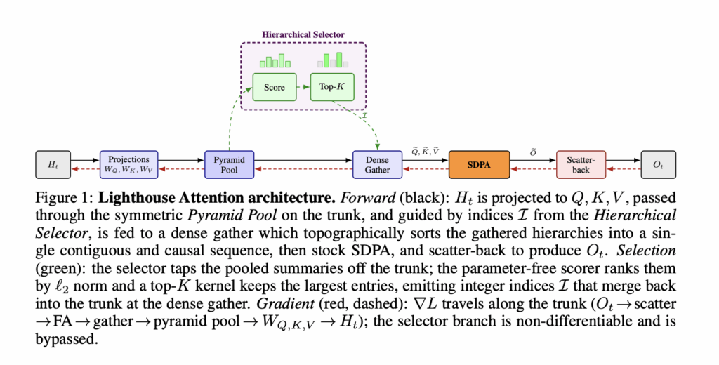
Training large language models on long sequences has a well-known problem: attention is expensive. The scaled dot-product attention (SDPA) at the core of every transformer scales quadratically Θ(N²) in both compute and memory with sequence length N. FlashAttention addressed this through IO-aware tiling that avoids materializing the full N×N attention matrix in high-bandwidth memory, reducing the memory footprint significantly, but the underlying Θ(N²) compute scaling remains. Researchers at Nous Research have introduced a new method called Lighthouse Attention that addresses this bottleneck specifically at pretraining time, achieving a 1.40× to 1.69× end-to-end wall-clock speedup against a cuDNN-backed SDPA baseline, with matching or lower final training loss. The core problem with existing sparse attention methods To understand why Lighthouse works the way it does, it helps to know what existing sparse attention methods do. Most prior work like NSA, HISA, DSA, MoBA makes the same two design decisions. First, they pool only the key and value side while leaving queries at full resolution (asymmetric compression). Second, their selection logic lives inside a custom attention kernel, which means teams can’t reuse the optimized dense-attention kernels that modern GPU tensor cores are built around. There is also a concern specific to training that inference-only sparse methods don’t face. An inference-time sparse method is evaluated only against its dense backbone and it is at most as good as that backbone. A training-time sparse method faces a harder test: once training is done, will the resulting weights still produce a competent dense-attention model at inference? Lighthouse treats that question as its central correctness criterion. Lighthouse takes a different approach on both design decisions. It pools queries, keys, and values symmetrically across a multi-level pyramid, and it places selection entirely outside the attention kernel. After selection, the system gathers the chosen entries into a contiguous, dense sub-sequence and runs stock FlashAttention on it — the same kernel used by the dense baseline. https://arxiv.org/pdf/2605.06554 How the four-stage pipeline works A Lighthouse attention layer wraps around, but does not modify, scaled dot-product attention. The pipeline has four stages. In the first stage, average pooling constructs an L-level pyramid from Q, K, and V. With pooling factor p, level ℓ of the pyramid has N/p^ℓ tokens, each summarizing p^ℓ base positions. Crucially, the same pooling applies to all three projections, producing coherent (Q^(ℓ), K^(ℓ), V^(ℓ)) triples at every level. Total pyramid construction costs Θ(N) time and memory. In the second stage, a parameter-free scorer assigns each pyramid entry two scalar scores using per-head ℓ₂ norms: one as a query score (∥Q^(ℓ)_i∥₂) and one as a key score (∥K^(ℓ)_i∥₂). Coarser levels inherit scores from finer ones via max-pooling, so a coarse span picks up the importance of its strongest token. A fused chunked-bitonic top-K kernel then selects k entries jointly across all pyramid levels. One design detail worth noting: the coarsest pyramid level is always retained in full — it is cheap and guarantees at least one contributor at every base position; the remaining selection budget is spent on finer levels. Additionally, the chunked-bitonic design produces a stratified top-K rather than a strict global top-K: the score stream is partitioned into fixed-size chunks, each maintaining an in-register top-m buffer, so if the k globally highest-scoring entries clustered in one chunk, some would be replaced by lower-scoring entries from other chunks. The result is more balanced attention coverage across the sequence and avoids selection collapse onto a narrow span. The top-K step is discrete and non-differentiable — no straight-through estimator, no Gumbel softmax. Selection indices carry no gradient. Gradients flow only through the gathered Q, K, V entries into WQ, WK, WV, so the projections learn to produce values that are useful when selected rather than scores that are good at selecting. In the third stage, the selected entries are gathered into a contiguous sub-sequence of length S = N/p^(L−1) + (L−1)·p·k and passed to standard FlashAttention. At N = 1,000,000 with L = 4, p = 4, k = 4,096, S ≈ 65,000 — far smaller than N. A critical property of the gathering process is that it guarantees no “holes” or empty spaces in the assembled sub-sequence. This matters specifically because Lighthouse also compresses queries: a gap in the sequence would mean those missing tokens have no gradient path during the backward pass and could cause training instabilities. Asymmetric methods that leave queries at full resolution don’t face this problem, but Lighthouse’s symmetric design requires that the gathered sub-sequence remains fully dense. In the fourth stage, each output entry is scattered back to the p^ℓ base positions it represents via a deterministic integer-atomic scatter kernel, with a shift of p^ℓ − 1 to preserve causality. The per-position fan-in is bounded by L regardless of k. https://arxiv.org/pdf/2605.06554 Why symmetric pooling changes the compute Pooling queries alongside keys and values changes the computational character of the attention call from O(N Sd) to O(S² d) at training time. Because S ≪ N at long contexts, this is what produces the latency advantage. Benchmarked on a single NVIDIA B200 at 512K context (bfloat16, B=1, H=8, head dimension 128, L=3, p=4, sparsity ≈ 1:64), Lighthouse is 21× faster on the forward pass and 17.3× faster on the combined forward+backward pass relative to cuDNN-backed SDPA. From an asymptotic standpoint, setting L = logp(N/k) gives a gathered sub-sequence size of S = Θ(k log N), which makes the dense FlashAttention call cost Θ(k² log² N d) — polylogarithmic in N at fixed k. Combined with the linear-cost stages (pyramid construction, scoring, scatter-back), total per-layer compute is Θ(T d) at bounded k — the same asymptotic class as linear attention and SSMs — while preserving softmax attention’s recall properties on the selected sub-sequence. Inference is a different constraint. Autoregressive decoding presents one query at a time, which violates the assumption that all queries co-occur in one forward pass. Lighthouse is a training-only method, and the symmetric pooling design cannot be used directly at inference. The two-stage training recipe and recoverability The experimental setup used a 530M-parameter

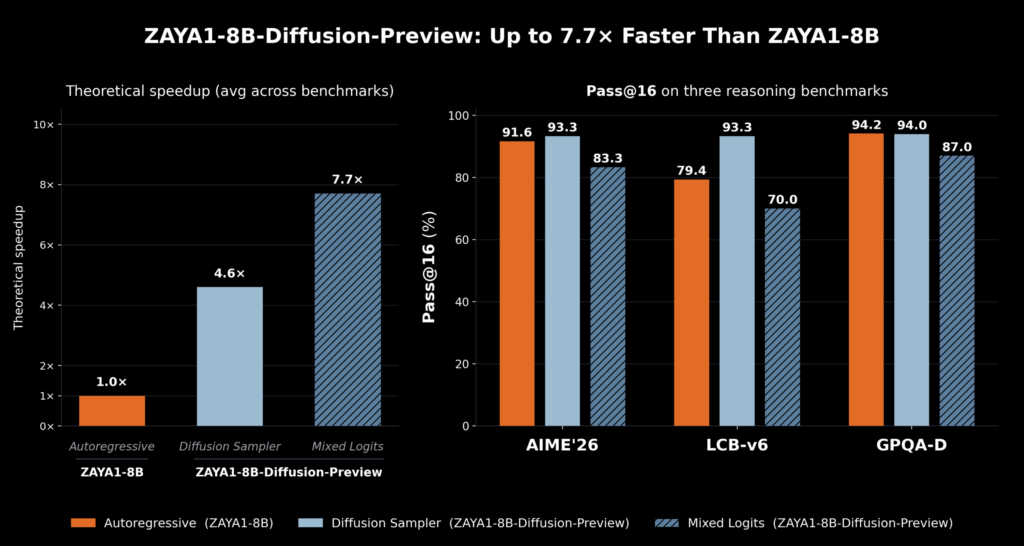
Zyphra, the San Francisco-based AI lab behind the ZAYA1 model family, released ZAYA1-8B-Diffusion-Preview — a preview of its early work in diffusion-language models. The release demonstrates that an existing autoregressive language model can be converted into a discrete diffusion model with no systematic loss of evaluation performance, while delivering substantial inference speedups on AMD hardware. https://www.zyphra.com/post/zaya1-8b-diffusion-preview The Problem With Autoregressive Decoding To understand why this matters, it helps to first understand how most language models generate text today. Standard large language models are autoregressive: they decode one token at a time in sequence. For each new token, the attention mechanism has to look back over all previously generated tokens and load their stored representations — called the KV-cache — from GPU memory. Crucially, because every user in a batch has a different history of tokens, each user’s KV-cache must be loaded separately and cannot be shared across requests. This creates a bottleneck. When the GPU spends more time moving data from memory than performing actual computation, the system becomes memory-bandwidth bound rather than compute-bound. This limits how efficiently modern GPU hardware — which has been scaling compute FLOPs faster than memory bandwidth — can be used during inference. Diffusion offers an alternative. Instead of generating one token at a time, a diffusion model generates multiple drafts of N tokens simultaneously and iterates this drafting process multiple times. Because all N tokens in the block share the same KV-cache, the operation shifts from memory-bandwidth bound to compute-bound, which means the GPU can be utilized more efficiently. In ZAYA1-8B-Diffusion-Preview specifically, the model performs a single-step transformation from mask to token for each token in the block — meaning it directly predicts the unmasked token in one step rather than iteratively denoising. Converting Autoregression to Diffusion Without Training From Scratch Training a diffusion language model from scratch is technically difficult, and there are few established recipes for doing so. Zyphra team offers two reasons for preferring conversion over training from scratch: first, it is simply hard, with few known recipes; second, there is no advantage to training in diffusion-mode because training is already compute-bound — the memory-bandwidth bottleneck that diffusion solves only appears at inference time. This means all the benefits of diffusion are inference-time benefits, and an existing pretraining stack can be reused as-is. Building on the TiDAR recipe, Zyphra took the ZAYA1-8B-base checkpoint and performed an additional 600 billion tokens of diffusion-conversion mid-training at a 32k context length, followed by 500 billion tokens of native context extension to 128k, and then a diffusion supervised fine-tuning (SFT) phase. ZAYA1-8B-Diffusion-Preview is the first MoE diffusion model converted from an autoregressive LLM, and the first diffusion-language model to be trained on AMD GPUs. Zyphra reports minimal evaluation degradation compared to the base autoregressive checkpoint, with gains on some benchmarks such as LCB-v6. They attribute this partly to improved mid-training datasets and partly to the greater expressivity of diffusion-style within-block non-causal inference compared to causal autoregression. How the Diffusion Sampler Works During inference, ZAYA1-8B-Diffusion-Preview generates a draft of 16 tokens simultaneously. A fraction of these tokens are accepted based on a sampling criterion borrowed from speculative decoding. The key advantage here is that the same model acts as both speculator and verifier within a single forward pass, which removes the overhead associated with running two separate models as in traditional methods like EAGLE or dFlash. In heavily memory-bandwidth-bound regimes, almost all accepted tokens represent free speedup over autoregressive decoding — the GPU is already loaded and the extra tokens cost very little additional compute. Zyphra team reports two samplers with different speed-quality trade-offs: Lossless diffusion sampler: Uses the standard speculative decoding acceptance criterion of min(1, p(x)/q(x)), where p is the autoregressive model’s logit distribution and q is the diffusion model’s distribution. Upon rejection, the next token is sampled from the residual distribution of p(x)-q(x). This sampler achieves a 4.6x speedup with no systematic evaluation degradation. Logit-mixing sampler: First mixes the logits from the diffusion speculator and the autoregressive model, then uses the averaged distribution for verification. This improves acceptance rates because the verification logits are closer to the diffusion logits, but has some impact on quality. This sampler achieves a 7.7x speedup. The trade-off between speed and quality can be chosen at runtime. One important caveat on these numbers: because ZAYA1-8B-Diffusion-Preview is a base mid-train checkpoint that has not yet undergone RL training, Zyphra uses pass@ evaluations rather than standard accuracy benchmarks to better represent the model’s ultimate potential after RL training. Readers comparing these figures to other models’ reported benchmarks should keep this in mind. Zyphra team also notes that the speedups observed from diffusion are higher than those from alternative methods such as multi-token prediction (MTP) and various speculative decoding strategies such as EAGLE3. Since TiDAR-style diffusion models utilize a single forward pass only, acceptance rates comparable to dFlash still yield substantial speedups. https://www.zyphra.com/post/zaya1-8b-diffusion-preview Architecture Details ZAYA1-8B-Diffusion-Preview is a single-step speculative diffusion model that uses order constrained generation which means the diffusion model is only capable of generating tokens in a contiguous subsequence starting from the prefix. This constraint increases training stability dramatically compared to unconstrained mask diffusion objectives or set block decoding, and was a primary reason Zyphra built on the TiDAR recipe. The model uses ZAYA1-8B’s existing CCA attention variant from Zyphra. CCA dramatically reduces prefill FLOPs in attention, which is directly beneficial for diffusion because diffusion converts decoding into a prefill-like operation. This means CCA lets the model diffuse more tokens in parallel before hitting compute limits. More specifically, the architecture uses CCGQA with a 4:1 ratio between query heads and key heads. One design choice behind this was deliberately avoiding MLA (Multi-Head Latent Attention), whose high arithmetic intensity was seen as a mismatch compared to CCGQA. Since block diffusion accesses the same cache, arithmetic intensity scales with block size and with the number of blocks per forward pass. On AMD MI300x hardware in bf16, the system supports roughly three block-sized proposals per single forward pass; on MI355x, this

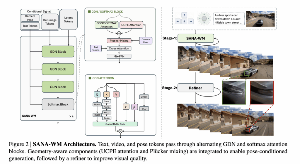
World models (systems that synthesize realistic video sequences from an initial image and a set of actions) are becoming central to embodied AI, simulation, and robotics research. The core challenge is scaling these systems to generate minute-long, high-resolution video without requiring prohibitively large clusters for both training and inference. Most competitive open-source baselines either require multi-GPU inference or sacrifice resolution to stay within compute budgets. NVIDIA’s SANA-WM directly targets these bottlenecks. Built on the SANA-Video codebase and available through the NVlabs/Sana GitHub repository, it is a 2.6B-parameter Diffusion Transformer (DiT) trained natively for one-minute generation at 720p with metric-scale 6-DoF camera control. It supports three single-GPU inference variants: a bidirectional generator for high-quality offline synthesis, a chunk-causal autoregressive generator for sequential rollout, and a few-step distilled autoregressive generator for faster deployment. The distilled variant denoises a 60-second 720p clip in 34 seconds on a single RTX 5090 with NVFP4 quantization. https://arxiv.org/pdf/2605.15178 The Architecture: Four Core Design Decisions 1. Hybrid Linear Attention with Gated DeltaNet (GDN) Standard softmax attention has memory and compute complexity that grows quadratically with sequence length — a serious problem when generating 961 latent frames for a 60-second video at 720p. SANA-Video, the predecessor, used cumulative ReLU-based linear attention, which maintains a constant-size recurrent state. However, this has no decay mechanism: all past frames accumulate with equal weight, causing drift over minute-scale sequences. SANA-WM replaces most attention blocks with frame-wise Gated DeltaNet (GDN). Unlike token-wise GDN used in language models, SANA-WM’s frame-wise variant processes one entire latent frame per recurrent step. The GDN update rule incorporates a decay gate γ (which down-weights stale past frames) and a delta-rule correction (which updates only the residual between the target value and the current state prediction), keeping the recurrent state at a constant D×D size regardless of video length. To stabilize training, the research team introduces an algebraic key-scaling approach: keys are scaled by 1/√(D·S), where D is the head dimension and S is the number of spatial tokens per frame. This ensures the spectral norm of the transition matrix remains bounded and eliminates the NaN divergence events observed with standard L2 key normalization (1/√D) or no scaling at all, both of which triggered NaN events at steps 16 and 1, respectively. The final backbone interleaves 15 frame-wise GDN blocks with 5 softmax attention blocks (at layers 3, 7, 11, 15, and 19) across 20 total transformer blocks. The softmax blocks provide exact long-range recall where GDN’s recurrence alone is insufficient. 2. Dual-Branch Camera Control Camera-controlled world modeling requires the model to faithfully follow a continuous 6-DoF trajectory, not just align with a text description of motion. SANA-WM uses two complementary branches that operate at different temporal rates: Coarse branch (UCPE attention): Operates at the latent-frame rate. For each latent token, it computes a ray-local camera basis from the camera-to-world pose and intrinsics, then applies a Unified Camera Positional Encoding (UCPE) to the geometric channels of each attention head. This captures global trajectory structure across the full sequence. Fine branch (Plücker mixing): Addresses a compression mismatch. Each latent token summarizes eight raw frames, each with its own distinct camera pose. The fine branch computes pixel-wise Plücker raymaps (a 6D representation: ray direction d and moment o×d) from all eight raw frames within one VAE temporal stride, packs them into a 48-channel tensor, and injects this embedding after each self-attention output via a zero-initialized projection. This restores intra-stride camera motion that the coarse branch cannot see at latent-frame resolution. Ablations on OmniWorld show that neither branch alone matches the dual approach: UCPE-only achieves a Camera Motion Consistency (CamMC) of 0.2453, while UCPE + Plücker mixing reaches 0.2047. 3. Two-Stage Generation Pipeline Stage-1 SANA-WM outputs, while spatiotemporally consistent, can contain structural artifacts over long sequences. A second-stage refiner, initialized from the 17B LTX-2 model with rank-384 LoRA adapters fine-tuned on paired synthetic and real video data, corrects these artifacts. It uses truncated-σ flow matching: stage-1 latents are perturbed with a large starting noise (σ_start = 0.9), and the refiner learns to map this noisy input toward the high-fidelity target. Only three Euler denoising steps are needed at inference. The refiner reduces long-horizon visual drift (ΔIQ) from 3.79 to 1.17 on the Simple-Trajectory split, and from 3.09 to 0.31 on the Hard-Trajectory split. 4. Robust Data Annotation Pipeline Training camera-controlled video generation requires metric-scale 6-DoF pose annotations, the information not available in standard video datasets. The research team modified VIPE (a camera-pose annotation engine) by replacing its depth backend with Pi3X (for long-sequence-consistent depth) fused with MoGe-2 (for accurate per-frame metric scale). They also extended the bundle adjustment stage to treat focal lengths and principal points as per-frame variables rather than shared global intrinsics, enabling more robust annotation on internet video with varying focal lengths. The resulting pipeline processes seven training corpus entries drawn from multiple open-source sources: SpatialVID-HQ (real, 10s clips), DL3DV real clips (10s), DL3DV GS Refined synthetic clips (60s, rendered via 3D Gaussian Splatting), OmniWorld (synthetic, 60s), Sekai Game (synthetic, 60s), Sekai Walking-HQ (real, 60s), and MiraData (real, 60s). This yields a total of 212,975 clips with metric-scale pose annotations. The LTX2-VAE used for compression is 2.0× smaller than ST-DC-AE and 8.0× smaller than Wan2.1-VAE, which directly improves training and inference efficiency. For DL3DV, which contains static 3D scene captures rather than native one-minute videos, the research team fit one FCGS 3D Gaussian Splatting reconstruction per scene, designed diverse one-minute camera paths, rendered long videos with known intrinsics and extrinsics, and then refined the rendered outputs with DiFix3D to reduce splatting artifacts. Training Strategy and Infrastructure SANA-WM’s compute involves two phases on 64 H100 GPUs. First, before DiT training, the team adapts the LTX2 VAE to the SANA-Video SFT training data in approximately 50K steps, taking roughly 3.5 days. The main DiT training then follows a four-stage progressive schedule lasting approximately 15 days: Stage 1 (~2.75 days): Adapt the pre-trained SANA-Video model to the frame-wise GDN architecture on short (5s) video clips. This replaces cumulative linear attention with the

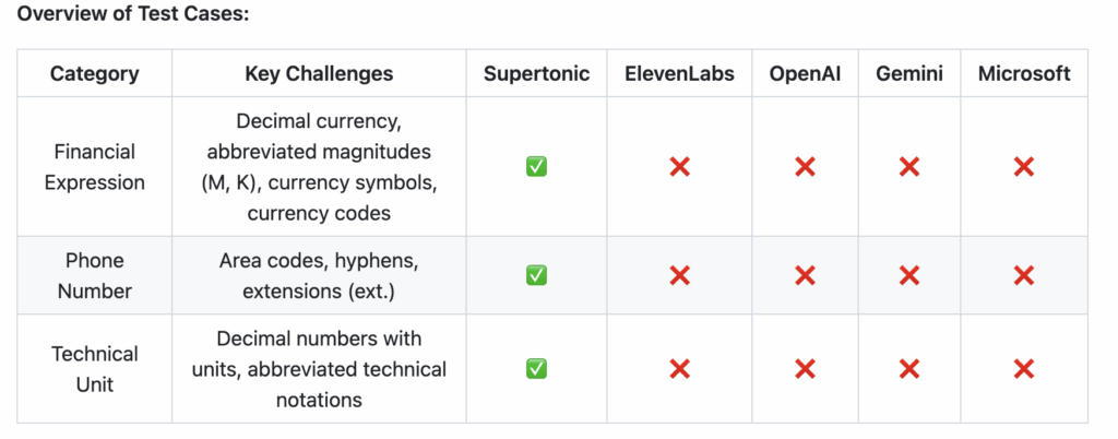
Supertone released Supertonic 3, the third generation of its on-device, ONNX-based text-to-speech system. Supertonic 3 ships with 31-language support, improved reading accuracy, fewer repeat and skip failures, and v2-compatible public ONNX assets. It is Lightning Fast, On-Device, Multilingual and Accurate TTS. What Changed from v2 to v3 Compared with Supertonic 2, Supertonic 3 reduces repeat and skip failures, improves speaker similarity across the shared-language set, and expands language coverage from 5 to 31 languages. Version 2 supported English, Korean, Spanish, Portuguese, and French. Version 3 adds Japanese, Arabic, Bulgarian, Czech, Danish, German, Greek, Estonian, Finnish, Croatian, Hungarian, Indonesian, Italian, Lithuanian, Latvian, Dutch, Polish, Romanian, Russian, Slovak, Slovenian, Swedish, Turkish, Ukrainian, and Vietnamese — 31 total ISO language codes. There is also a special na fallback for text whose language is unknown or outside the supported set. The model grows modestly to accommodate the added languages. At about 99M parameters across the public ONNX assets, Supertonic 3 is much smaller than 0.7B to 2B class open TTS systems. The smaller model size is a practical advantage for download size, startup time, and on-device inference. The update also brings the total disk footprint of the public ONNX assets to 404 MB. Additionally, Supertone recently launched the Voice Builder, allowing developers to create custom, edge-native TTS models from their own voice recordings. Expressive Tags One new capability in v3 that wasn’t present in v2 is expressive tag support. Supertonic 3 supports simple expression tags such as <laugh>, <breath>, and <sigh>. These let you embed prosodic cues directly into input text without a separate preprocessing step or a separate model for expressiveness. For engineers building voice interfaces or accessibility tools, this means you can specify breathing pauses or laughter inline in your text payload. Architecture and Runtime The underlying architecture carries over from prior versions: a speech autoencoder that encodes waveforms into continuous latent representations, a flow-matching based text-to-latent module that maps text to audio features, and a duration predictor that controls natural timing. Flow matching is a generative modeling technique that learns a vector field to transform a simple distribution into a target distribution — it samples faster than diffusion models at low step counts, which is why Supertonic can produce usable output in just 2 inference steps. To further refine output, v3 integrates Length-Aware Rotary Position Embedding (LARoPE) for superior text-speech alignment and utilizes a Self-Purifying Flow Matching technique during training to remain robust against noisy data labels. On runtime efficiency, Supertonic 3 runs fast on CPU, even compared with larger baselines measured on A100 GPU, and uses substantially less memory. It does not require a GPU, which makes local, browser, and edge deployment much easier. Reading Accuracy Across measured languages, Supertonic 3 stays within a competitive WER/CER range against much larger open TTS models such as VoxCPM2, while preserving a lightweight on-device deployment path. WER (Word Error Rate) and CER (Character Error Rate) are standard TTS readability metrics: you synthesize a passage, run ASR over the output, and compare the transcription to the original text. CER is used for languages without clear word boundaries; the others use WER. The system’s efficiency is best demonstrated on extreme edge hardware; it achieves an average RTF of 0.3x on an Onyx Boox Go 6 (an E-ink e-reader) in airplane mode. Furthermore, the ecosystem has expanded to include Flutter (with macOS support), .NET 9, and Go, while the web implementation leverages onnxruntime-web for pure client-side execution. Text Normalization A differentiating property carried forward from v2 is built-in text normalization. Supertonic handles complex surface forms — financial expressions like $5.2M, phone numbers with area codes and extensions like (212) 555-0142 ext. 402, time and date formats like 4:45 PM on Wed, Apr 3, 2024, and technical units like 2.3h and 30kph — without any preprocessing pipeline or phonetic annotations. The financial expression “$5.2M” must read as “five point two million dollars,” and “$450K” as “four hundred fifty thousand dollars.” All four competing systems failed this. The technical unit “2.3h” must read as “two point three hours” and “30kph” as “thirty kilometers per hour.” All four competitors also failed this category. The competing systems evaluated include ElevenLabs Flash v2.5, OpenAI TTS-1, Gemini 2.5 Flash TTS, and Microsoft. https://github.com/supertone-inc/supertonic Getting Started The Python SDK install is pip install supertonic. On first run, the SDK downloads the model assets from Hugging Face automatically. A minimal example: Copy CodeCopiedUse a different Browser from supertonic import TTS tts = TTS(auto_download=True) style = tts.get_voice_style(voice_name=”M1″) text = “A gentle breeze moved through the open window while everyone listened to the story.” wav, duration = tts.synthesize(text, voice_style=style, lang=”en”) tts.save_audio(wav, “output.wav”) print(f”Generated {duration:.2f}s of audio”) Marktechpost’s Visual Explainer Supertonic 3 — Developer Guide 1 / 7 Overview Supertonic 3: On-Device TTS,Now in 31 Languages Supertonic 3 is a lightweight, open-weight text-to-speech system by Supertone Inc. It runs entirely via ONNX Runtime on your device — no cloud, no API call, no data leaving your machine. v3 expands from 5 to 31 languages, adds expressive tags, reduces reading failures, and stays compatible with the v2 ONNX interface. 31 Languages ~99M Parameters 404 MB ONNX Assets MIT Code License What’s New in v3 Four Core Improvements Over Supertonic 2 Version 3 is a focused upgrade — same inference contract, meaningfully better output. 31 languages — Expanded from the 5-language v2 release (en, ko, es, pt, fr). Now includes Japanese, Arabic, German, Hindi, Russian, Turkish, Vietnamese, and 20 more ISO codes, plus a special na fallback for unknown languages. More stable reading — Fewer repeat and skip failures, especially on short and long utterances. This was a known limitation in v2 that v3 directly addresses. Expression tags — Supports <laugh>, <breath>, and <sigh> inline in text, without any separate preprocessing or external model. Higher speaker similarity — Improved similarity across the shared-language set compared with Supertonic 2. Voices are more consistent across languages. Installation Get Running in Under a Minute Install the Python SDK via pip. On first run, model assets are downloaded automatically from Hugging Face