Uncategorized

Throughout 2025, HPE observed significant changes in how cybercriminals operate. Analyzing real-world threats, our HPE Threat Labs highlighted an industrialization of the cyber criminals’ methods in its new In the Wild Report, enabling greater scale, speed and structure in their campaigns. They typically use automation and AI to exploit longstanding vulnerabilities, and many have adopted a professional, corporate hierarchy to optimize their efficiency. Cybersecurity threats today are as menacing as ever for enterprises, as any CISO or CIO can probably confirm. But, digging behind that straightforward statement, there is a much more nuanced, complex cybersecurity landscape at play. This can make it significantly harder to plan, execute, and sustain effective strategies and solutions to protect the network—plus the often valuable—sometimes priceless—data, apps, and assets it transports and stores. But it can be done, with the right philosophy and strategy, and the right tools and insights. We must first understand the contemporary cybersecurity landscape. This understanding can unlock the right strategy and then onward to identify the tools and insights necessary to protect an enterprise’s network effectively. There are five primary factors influencing the landscape, some old, some new, all dynamic. These factors are distinct but often interdependent, both within themselves and with one or more of the others. Another meaningful way of looking at them is “internal” and “external”; as ever, understanding and dealing with what is in your control can also help to navigate and mitigate what is beyond your control. Five key factors influencing today’s dynamic cybersecurity landscape 1. Expectations The first factor is predicated on the fundamental reality of an enterprise’s reliance on its network. Most enterprises have already undergone some form of digital transformation and are reaping the day-to-day benefits. This means that the number of people, devices, and things using the network continues to grow; it also means that people’s expectations of the network are higher than ever before – they demand that it does exactly what they need it to do, typically across a proliferation of devices and from multiple locations. Conversely, many employees might not be fully aware of cyber threats and infiltration methods, so their skillsets can easily be the weak point that admits bad actors into the network. Equally, senior management and board members have high expectations at a meta level. Embracing digital transformation and network reliance means the enterprise’s function and reputation are inextricably tied to that. Loss of reputation due to a security breach is a chilling prospect, as is the threat of financial penalty and revenue loss. So, in the minds of leadership, the network has to be safe from cyber threats and be compliant. 2. Financial pressures The first factor arguably contradicts its neighbor in the landscape: general financial constraints and the pressure on CISOs and CIOs to achieve more with less. Despite the strategic reliance on the network and the expectation that it will be protected from cyber threats regardless, the appropriate latticework of defenses (e.g., skilled and right-sized IT teams using progressive tools and meaningful data insights, plus constant workforce education) is not always properly funded and sustained, particularly in the current tough economic climate. 3. Complex infrastructure operations The ongoing pursuit of digital transformation and consequent network reliance also drives the third factor. Ironically, there is another facet of enterprise protection and financial control wrapped up in this. The widespread move from one-stop shops (avoiding IT vendor lock-in in favor of more competitive pricing and autonomy) has created a more complex, multivendor environment. This is coupled with multiple IT domains required to handle many diverse functions and layers of IT infrastructure (e.g., cloud, on-prem), all connected to the network. Complex, mission-critical IT operations now need to be monitored and protected from increasingly sophisticated cyber breaches. 4. Unpredictable geopolitics and economics Shifting from the first three factors—all internal to an enterprise—the fourth is unquestionably external and without doubt the most intractable risk for any enterprise, individual, or industry group. Global uncertainty and tension are unavoidably putting even greater pressure on already-tight IT budgets, component supply chains and power costs. This can easily exacerbate existing constraints on cybersecurity budgets when vigilance and protection are more needed than ever. Unfortunately, in cyberspace one cannot always point a finger in one direction to identify an adversary. Geopolitical alliances in cyberspace are much more difficult to track, and defending against an escalating tension becomes an all-out fight to secure the network. 5. Evolving cyber threats The fifth factor is obviously the epicenter of today’s cyber security landscape. According to the HPE Threat Labs’ report, governments were the most frequently targeted sector globally in 2025, followed by finance, technology, defense, and manufacturing. The prevailing global geopolitical and economic situation may further accelerate the twin motivations of nation state-linked espionage and organized crime for extortion and theft. Use the network to protect the network… and beyond The current cybersecurity landscape calls for a re-think of the network’s pivotal role and how it can manage an enterprise’s digital defenses effectively, dynamically, and comprehensively. Overall, the network can be an excellent security sensor and enforcement point, using built-in security capabilities rather than being a collection of devices with an inflexible, bolted-on security layer. Much as cybercriminals use agentic and generative AI to intensify their campaigns, CISOs can stay ahead more easily by leveraging AI-driven network platforms for 24×7 automated management of security policy enforcement (e.g., zero trust), threat monitoring, and mitigation, encompassing devices, things, and users. Meaningful data insights can be harvested, analyzed, and recycled back into secure networking management tools for dynamic protection. This approach helps the progressive enterprise to overcome increasingly sophisticated, multi-step, and prolific attacks, while better managing IT costs and simplifying oversight of IT operations. It can also significantly improve the user experience, going a long way to meet and even exceed those rising expectations consistently.  As a strategy in today’s uncertain world, embracing this self-driving network paradigm enables flexibility, visibility, and consistency in an enterprise’s frontline digital defenses. For more, read the “In the Wild” report. This

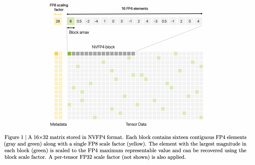
Pretraining frontier-scale LLMs in FP8 is now standard practice, but moving to 4-bit floating point has remained an open research problem because narrower formats compress dynamic range and amplify quantization error at long token horizons. A new research from NVIDIA describes a pretraining methodology built around NVFP4, a 4-bit microscaling format supported natively by Blackwell Tensor Cores, and validates it by pretraining a 12-billion-parameter hybrid Mamba-Transformer on 10 trillion tokens. The research team state this is the longest publicly documented training run in 4-bit precision to date. The resulting model attains 62.58% on MMLU-Pro 5-shot versus 62.62% for the FP8 baseline, and is supported in NVIDIA’s Transformer Engine. What NVFP4 Actually is To understand why NVFP4 is important, it helps to revisit how microscaling formats work. In a microscaling (MX) format, a contiguous block of low-precision elements shares a single scale factor, which is used to map the block back into a wider numerical range during the matrix multiply. MXFP4 uses 32-element blocks where each element is stored as E2M1 — 1 sign bit, 2 exponent bits, 1 mantissa bit — encoding only the values ±0, ±0.5, ±1, ±1.5, ±2, ±3, ±4, and ±6. Block scale factors are stored in UE8M0, which restricts them to powers of two. NVFP4 changes three things. First, the block size drops from 32 to 16 elements, narrowing the dynamic range each scale has to cover. Second, block scale factors are stored in E4M3 rather than UE8M0, trading exponent range for mantissa precision so the per-block amax (absolute maximum) can be mapped much closer to the FP4 maximum representable. Third, NVFP4 adds a second scaling level: an FP32 per-tensor scale that remaps values so the E4M3 block scales themselves stay in range. The result is that at least 6.25% of values in each block — the per-block amax — are represented at near-FP8 precision, while the remainder sit in FP4. On NVIDIA Blackwell, FP4 GEMMs run at 4× BF16 throughput on GB200 and 6× on GB300, which translates to roughly 2× and 3× speedups over FP8. Operand memory footprint is approximately halved compared to FP8. https://arxiv.org/pdf/2509.25149 What’s Quantized — and What Isn’t Only the GEMMs inside linear (fully-connected) layers Fprop, Dgrad, and Wgrad actually run in NVFP4. Embeddings, the output projection head, normalization layers, non-linearities, and all attention components (softmax and the query-key and attention score-value batched GEMMs) stay in BF16 or FP32. Model weights, weight gradients used for accumulation across microbatches and data-parallel replicas, and optimizer states are kept in FP32. Tensor parallel reductions run in BF16. The Four-Part Training Methodology Quantizing every linear-layer GEMM to NVFP4 with default settings (1×16 block scaling everywhere, round-to-nearest-even on every tensor, no transforms) diverges early in training. NVIDIA’s approach stabilizes it with four components, and ablation studies on the 12B model show each is necessary. Selective high precision: Linear layers in the first two and the final eight of the 62 blocks (about 16% of all linear layers) are kept in BF16. Ablations indicated that the final blocks are the sensitive ones because they require more dynamic range than FP4 provides; keeping only the final four blocks in BF16 was also enough for stable convergence. Random Hadamard Transforms (RHT): Outliers in weight gradients are spread into an approximately Gaussian distribution by multiplying the input tiles with a 16×16 Hadamard matrix combined with a random ±1 sign vector. Because the orthogonal transforms cancel inside the dot-product, no math correction is needed in the GEMM. The d=16 size was chosen empirically: d=4 hurt convergence, d=128 gave similar results. RHT is applied only to the inputs of the weight-gradient (Wgrad) GEMM, and a single random sign vector is shared across all linear layers. Randomization itself was a no-op at the 1.2B scale but measurably improved the 12B run. Two-dimensional (2D) block scaling for weights: Standard NVFP4 scales 1×16 blocks along the dot-product dimension. Because the backward pass transposes the weight tensor, the forward and backward passes end up with different quantized weights, breaking the chain rule. NVIDIA’s fix is to scale weights in 16×16 blocks so the same quantized representation is used in both passes. Activations and gradients keep 1×16 scaling, since they are less sensitive to this inconsistency. Stochastic rounding on gradients: Round-to-nearest-even introduces systematic bias when applied to gradient tensors. Stochastic rounding rounds probabilistically based on distance to the two nearest representable values, removing that bias. The research team explicitly notes in research paper that stochastic rounding is detrimental when applied to forward-pass tensors, so it is restricted to gradients. Results on the 12B Hybrid Mamba-Transformer The 12B model uses the Nemotron-Nano-12B-v2-Base architecture — 62 blocks (6 Self-Attention, 28 FFN, 28 Mamba-2), hidden dimension 5120, FFN dimension 20480 — trained with a Warmup-Stable-Decay schedule (constant LR through 80% of training, decay over the final 20%), batch size 736, sequence length 8192. The FP8 reference baseline follows the DeepSeek-V3 methodology: E4M3 elements, 128×128 weight blocks, 1×128 activation and gradient blocks, with the first block and last two blocks kept in BF16. NVFP4 validation loss stays within 1% of the FP8 baseline during the stable phase and widens to slightly above 1.5% during decay. Downstream accuracy is comparable across most benchmarks: MMLU 76.57% vs 77.36%, GSM8K CoT 92.27% vs 89.08%, MATH 81.48% vs 83.32%, AGIEval English CoT 70.31% vs 67.01%. Coding shows the largest gap — HumanEval+ 57.43% vs 59.93%, MBPP+ 55.91% vs 59.11% — which the research team attributes partly to noisy final-checkpoint evaluation. The research team also documents a precision-switching technique: transitioning the forward pass from NVFP4 to BF16 starting at 8.2T tokens (about 18% of the schedule) reduced relative loss error from 1.5% to 0.5%. NVFP4 vs MXFP4 On a separate 8B hybrid Mamba-Transformer trained on 1T tokens, NVFP4 reached a relative loss error of about 1.5% versus BF16, while MXFP4 stayed near 2.5%. To close the gap, MXFP4 required 1.36T tokens to match the NVFP4 1T-token loss — a 36% token overhead. The research team attributes the difference to NVFP4’s smaller block size and E4M3

Search works well when users know exactly what they are looking for, but it breaks down when intent is described in natural language.

This is today’s edition of The Download, our weekday newsletter that provides a daily dose of what’s going on in the world of technology. Musk v. Altman week 3: Musk and Altman traded blows over each other’s credibility. Now the jury will pick a side. In the final week of the Musk v. Altman trial, lawyers attacked the credibility of the two tech leaders. Sam Altman was accused of lying and self-dealing, while Elon Musk was portrayed as a power-seeker trying to control artificial general intelligence. The case unearthed new details about the two arch-rivals and OpenAI’s contested nonprofit status, as well as a golden trophy of a donkey’s ass awarded to an employee who challenged Musk. Read the full story on the explosive final week of the trial. —Michelle Kim Michelle Kim, who’s also a lawyer, has been in court throughout the Musk v. Altman trial. Read her coverage of week 1 and week 2, plus a Q&A on what it was like in the room.  The must-reads I’ve combed the internet to find you today’s most fun/important/scary/fascinating stories about technology. 1 Trump traded hundreds of millions in tech stocks before favorable policy movesHe bought shares in Nvidia, AMD, and Arm ahead of policy boosts. (Quartz)+ And touted Palantir on Truth Social after buying its stock. (CNBC)+ His crypto venture and Iran’s top exchange tapped the same networks. (Reuters $) 2 SpaceX plans to list on the Nasdaq stock exchange as soon as June 12It wants to raise up to $75 billion at a $1.75 trillion valuation. (Reuters $)+ BlackRock may invest up to $10 billion in the offering. (The Information $)+ Cerebras’ blockbuster IPO has boosted hopes for the listing. (CNBC)+ Which is set to dwarf many of the biggest IPOs on ⁠record. (Reuters) 3 Chinese AI groups have pulled ahead of US rivals in video generationByteDance and Kuaishou’s models lead in realism and scale. (FT $)+ AI is fueling China’s short-drama boom. (MIT Technology Review)+ While its AI labs are betting big on open source. (MIT Technology Review) 4 Iran says it will charge Big Tech for using undersea internet cablesThe cables beneath the Strait of Hormuz carry vast digital traffic. (CNN)+ Tech bosses met at Uber HQ on Saturday to discuss Iran’s future. (404 Media) 5 Samsung has a “last chance” to stop a massive strike over AIOver 45,000 employees could walk out for 18 days this week. (CNBC) + They want a bigger share of the AI boom. (FT $)+ Samsung and its largest labor union will resume talks on Tuesday. (Reuters $) 6 Old oil and gas wells could become a new source of clean energyUS states plan to convert them into geothermal energy assets. (Wired $)+ A balcony solar boom is coming to the US. (MIT Technology Review) 7 The ChatGPT era has triggered a 30% surge in grades at a top universityGrades inflated in text-heavy courses but remained flat in others. (Axios)+ Princeton has changed its honor code because of AI cheating. (WSJ $)+ And real cheating rates may be far higher. (The Times $) 8 Ex-Google CEO Eric Schmidt was fiercely booed during an AI speechHis graduation speech praising AI agents sparked uproar. (The Verge)+ A populist backlash is building against AI. (MIT Technology Review) 9 Arm faces a US antitrust probe over its chip tech licensesRegulators are investigating whether it has an illegal monopoly. (Bloomberg $)+ Qualcomm has accused Arm of anticompetitive conduct. (Reuters $) 10 ArXiv will ban researchers who submit AI slopOffending authors face year-long bans from the pre-print server. (TechCrunch) Quote of the day “When someone offers you a seat on the rocket ship, you do not ask which seat. You just get on.”  —Ex-Google CEO Eric Schmidt extolls the virtues of AI agents in a graduation speech at the University of Arizona, prompting a chorus of boos. One More Thing WYSS INSTITUTE AT HARVARD UNIVERSITY Is this the end of animal testing? In a clean room in his lab, Sean Moore peers through a microscope at a bit of human intestinal tissue growing on a plastic chip. It’s one of 24 so-called “organs-on-chips” his team bought three years ago. The technology is designed to mimic human biology—and could reduce the need for animal testing. The appeal is not only ethical. Around 95% of drugs developed through animal research ultimately fail in people, and early studies suggest organ-on-a-chip systems may offer more accurate insights into how diseases behave and how drugs work. But the field still faces major technical and cost challenges before it can replace animal research. Find out how organ-on-chip technology could reshape drug testing. —Harriet Brown We can still have nice things A place for comfort, fun, and distraction to brighten up your day. (Got any ideas? Drop me a line.) + Listen to the captivating first recordings of whale songs from 1949.+ Meet the feline guardians of New York’s corner stores in this photo collection.+ A newly discovered floor plan allowed historians to pinpoint the location of Shakespeare’s only property in London.+ A music fan spent decades secretly recording 10,000 local shows. Now the entire collection is available online.

This is today’s edition of The Download, our weekday newsletter that provides a daily dose of what’s going on in the world of technology. Musk v. Altman week 3: Musk and Altman traded blows over each other’s credibility. Now the jury will pick a side. In the final week of the Musk v. Altman trial, lawyers attacked the credibility of the two tech leaders. Sam Altman was accused of lying and self-dealing, while Elon Musk was portrayed as a power-seeker trying to control artificial general intelligence. The case unearthed new details about the two arch-rivals and OpenAI’s contested nonprofit status, as well as a golden trophy of a donkey’s ass awarded to an employee who challenged Musk. Read the full story on the explosive final week of the trial. —Michelle Kim Michelle Kim, who’s also a lawyer, has been in court throughout the Musk v. Altman trial. Read her coverage of week 1 and week 2, plus a Q&A on what it was like in the room.  The must-reads I’ve combed the internet to find you today’s most fun/important/scary/fascinating stories about technology. 1 Trump traded hundreds of millions in tech stocks before favorable policy movesHe bought shares in Nvidia, AMD, and Arm ahead of policy boosts. (Quartz)+ And touted Palantir on Truth Social after buying its stock. (CNBC)+ His crypto venture and Iran’s top exchange tapped the same networks. (Reuters $) 2 SpaceX plans to list on the Nasdaq stock exchange as soon as June 12It wants to raise up to $75 billion at a $1.75 trillion valuation. (Reuters $)+ BlackRock may invest up to $10 billion in the offering. (The Information $)+ Cerebras’ blockbuster IPO has boosted hopes for the listing. (CNBC)+ Which is set to dwarf many of the biggest IPOs on ⁠record. (Reuters) 3 Chinese AI groups have pulled ahead of US rivals in video generationByteDance and Kuaishou’s models lead in realism and scale. (FT $)+ AI is fueling China’s short-drama boom. (MIT Technology Review)+ While its AI labs are betting big on open source. (MIT Technology Review) 4 Iran says it will charge Big Tech for using undersea internet cablesThe cables beneath the Strait of Hormuz carry vast digital traffic. (CNN)+ Tech bosses met at Uber HQ on Saturday to discuss Iran’s future. (404 Media) 5 Samsung has a “last chance” to stop a massive strike over AIOver 45,000 employees could walk out for 18 days this week. (CNBC) + They want a bigger share of the AI boom. (FT $)+ Samsung and its largest labor union will resume talks on Tuesday. (Reuters $) 6 Old oil and gas wells could become a new source of clean energyUS states plan to convert them into geothermal energy assets. (Wired $)+ A balcony solar boom is coming to the US. (MIT Technology Review) 7 The ChatGPT era has triggered a 30% surge in grades at a top universityGrades inflated in text-heavy courses but remained flat in others. (Axios)+ Princeton has changed its honor code because of AI cheating. (WSJ $)+ And real cheating rates may be far higher. (The Times $) 8 Ex-Google CEO Eric Schmidt was fiercely booed during an AI speechHis graduation speech praising AI agents sparked uproar. (The Verge)+ A populist backlash is building against AI. (MIT Technology Review) 9 Arm faces a US antitrust probe over its chip tech licensesRegulators are investigating whether it has an illegal monopoly. (Bloomberg $)+ Qualcomm has accused Arm of anticompetitive conduct. (Reuters $) 10 ArXiv will ban researchers who submit AI slopOffending authors face year-long bans from the pre-print server. (TechCrunch) Quote of the day “When someone offers you a seat on the rocket ship, you do not ask which seat. You just get on.”  —Ex-Google CEO Eric Schmidt extolls the virtues of AI agents in a graduation speech at the University of Arizona, prompting a chorus of boos. One More Thing WYSS INSTITUTE AT HARVARD UNIVERSITY Is this the end of animal testing? In a clean room in his lab, Sean Moore peers through a microscope at a bit of human intestinal tissue growing on a plastic chip. It’s one of 24 so-called “organs-on-chips” his team bought three years ago. The technology is designed to mimic human biology—and could reduce the need for animal testing. The appeal is not only ethical. Around 95% of drugs developed through animal research ultimately fail in people, and early studies suggest organ-on-a-chip systems may offer more accurate insights into how diseases behave and how drugs work. But the field still faces major technical and cost challenges before it can replace animal research. Find out how organ-on-chip technology could reshape drug testing. —Harriet Brown We can still have nice things A place for comfort, fun, and distraction to brighten up your day. (Got any ideas? Drop me a line.) + Listen to the captivating first recordings of whale songs from 1949.+ Meet the feline guardians of New York’s corner stores in this photo collection.+ A newly discovered floor plan allowed historians to pinpoint the location of Shakespeare’s only property in London.+ A music fan spent decades secretly recording 10,000 local shows. Now the entire collection is available online.

Running AI agents in a local script is straightforward. Running them reliably in production across teams, across restarts, with isolated environments per context is a different problem entirely. BerriAI, the company behind the LiteLLM AI Gateway, is now open-sourcing a purpose-built answer to that problem: the LiteLLM Agent Platform. The platform is described as a simple, self-hosted infrastructure platform for running multiple agents in production. What Problem Does it Solve? It helps to understand what happens when you try to scale agents beyond a single process. Agents are stateful: they carry session history, tool call results, and intermediate reasoning across turns. If the container running your agent crashes, restarts, or gets replaced during a deployment, that session state is gone unless something is explicitly managing it. At the same time, different teams often need different runtime environments, different tools, different secrets, different access scopes which means you cannot throw all agents into one shared container. The platform manages two things: per-team and per-context sandboxes, and session continuity across pod restarts and upgrades. These two capabilities are the core infrastructure primitives the platform provides. Architecture and Technical Stack The platform is a standalone Next.js dashboard for LiteLLM v2 managed agents, covering sessions chat, agent CRUD, and live status. The codebase is primarily TypeScript (92.8%), with Shell scripts for provisioning, a Dockerfile for containerization, and CSS for the dashboard UI. The architecture separates concerns cleanly. A web process runs on port 3000 and serves the Next.js dashboard. A worker process handles async agent tasks. Postgres is used as the persistent backing store, and a schema migration runs as an init container on startup — so the database is always in the correct state before the application boots. For the sandbox layer — the isolated runtime environment where agents actually execute — sandboxes run on Kubernetes via the kubernetes-sigs/agent-sandbox CRD. Local development uses kind. If you are not already familiar with it: kind (Kubernetes in Docker) lets you spin up a full Kubernetes cluster locally using Docker containers as nodes, without needing a cloud provider. The agent-sandbox CRD (Custom Resource Definition) is a Kubernetes extension from kubernetes-sigs that the platform installs to manage the lifecycle of individual sandbox environments. The platform also includes a harness system under harnesses/opencode, which contains the configuration for running coding agents — such as Claude Code or OpenAI Codex — inside isolated sandboxes with a vault proxy for credential management. BerriAI team also maintains a separate litellm-agent-runtime repository, described as a coding-agent runtime that runs inside per-session VMs provisioned by a LiteLLM proxy, generic by design, with customization happening via harness configuration or a hydrate payload. One practical detail worth noting is how environment variables are handled across sandbox containers. Anything in .env prefixed with CONTAINER_ENV_ is injected into every sandbox container with the prefix stripped — for example, CONTAINER_ENV_GITHUB_TOKEN=ghp_… means the container sees GITHUB_TOKEN=ghp_… This gives teams a clean way to pass secrets into sandboxed agent sessions without modifying container images. https://github.com/BerriAI/litellm-agent-platform Getting Started The prerequisites for local development are Docker Desktop, kind, kubectl, helm, and a LiteLLM gateway. No cloud credentials are required to get started locally. The quickstart is two commands: Copy CodeCopiedUse a different Browser bin/kind-up.sh docker compose up bin/kind-up.sh is idempotent — it provisions a kind cluster named agent-sbx, installs the agent-sandbox controller, and loads the harness image. docker compose up boots Postgres, runs the schema migration, and starts the web process on port 3000 along with the worker. For production deployment, the recommended path is AWS EKS for the sandbox cluster and Render for the web and worker processes. bin/eks-up.sh provisions the EKS cluster, and a Render Blueprint provides a one-click deployment option. Relationship to the LiteLLM Gateway The Agent Platform is a layer on top of the existing LiteLLM ecosystem, not a replacement for it. LiteLLM’s core is a Python SDK and Proxy Server — an AI Gateway — that calls 100+ LLM APIs in OpenAI format, with cost tracking, guardrails, load balancing, and logging, supporting providers including Bedrock, Azure, OpenAI, VertexAI, Cohere, Anthropic, SageMaker, HuggingFace, vLLM, and NVIDIA NIM. The Agent Platform consumes a running LiteLLM gateway as a dependency and builds agent orchestration and session management infrastructure on top of it. Model routing, cost tracking, and rate limiting remain in the gateway layer. Sandbox isolation, session continuity, and the management dashboard are handled by the Agent Platform. Marktechpost’s Visual Explainer LiteLLM Agent Platform Self-Hosted Agent Infrastructure Guide Alpha Overview Concepts Architecture Prerequisites Quickstart Production 01 / 06 What is LiteLLM Agent Platform? BerriAI open-sourced this platform on May 8, 2026. It is a self-hosted infrastructure layer for running multiple AI agents in production, built on top of the LiteLLM AI Gateway. Self-Hosted Runs entirely on your own infrastructure. No data leaves your environment. Suited for regulated industries and teams with data residency requirements. Multi-Agent Designed to run multiple agents in parallel, with full isolation between teams and contexts using per-session sandboxes. Session Continuity Agent sessions persist across pod restarts and upgrades, so stateful work is not lost when containers are replaced. Open Source (MIT) Fully open source under the MIT license. Repo: github.com/BerriAI/litellm-agent-platform. File issues and contribute directly. Prerequisite Knowledge This guide assumes familiarity with Docker, basic command-line usage, and a general understanding of what an AI agent is (a model that calls tools and runs multi-step tasks). Kubernetes experience helps but is not required to follow along. 02 / 06 Key Concepts to Know First Before running the platform, understand these four building blocks. They appear throughout the setup and configuration. A LiteLLM Gateway The underlying AI Gateway that the Agent Platform depends on. It routes requests to 100+ LLM providers (OpenAI, Anthropic, Bedrock, VertexAI, etc.) using a unified OpenAI-format API. The Agent Platform does not include the gateway, you must have one running separately and point the platform at it. B Sandbox An isolated container environment where a single agent session executes. Each sandbox is independent, meaning one agent cannot access the filesystem, secrets, or state

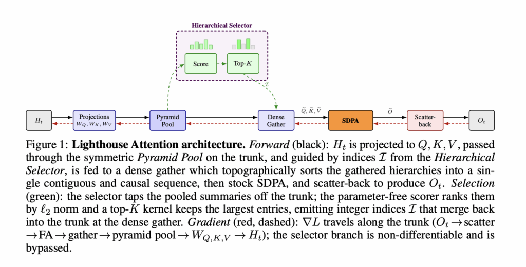
Training large language models on long sequences has a well-known problem: attention is expensive. The scaled dot-product attention (SDPA) at the core of every transformer scales quadratically Θ(N²) in both compute and memory with sequence length N. FlashAttention addressed this through IO-aware tiling that avoids materializing the full N×N attention matrix in high-bandwidth memory, reducing the memory footprint significantly, but the underlying Θ(N²) compute scaling remains. Researchers at Nous Research have introduced a new method called Lighthouse Attention that addresses this bottleneck specifically at pretraining time, achieving a 1.40× to 1.69× end-to-end wall-clock speedup against a cuDNN-backed SDPA baseline, with matching or lower final training loss. The core problem with existing sparse attention methods To understand why Lighthouse works the way it does, it helps to know what existing sparse attention methods do. Most prior work like NSA, HISA, DSA, MoBA makes the same two design decisions. First, they pool only the key and value side while leaving queries at full resolution (asymmetric compression). Second, their selection logic lives inside a custom attention kernel, which means teams can’t reuse the optimized dense-attention kernels that modern GPU tensor cores are built around. There is also a concern specific to training that inference-only sparse methods don’t face. An inference-time sparse method is evaluated only against its dense backbone and it is at most as good as that backbone. A training-time sparse method faces a harder test: once training is done, will the resulting weights still produce a competent dense-attention model at inference? Lighthouse treats that question as its central correctness criterion. Lighthouse takes a different approach on both design decisions. It pools queries, keys, and values symmetrically across a multi-level pyramid, and it places selection entirely outside the attention kernel. After selection, the system gathers the chosen entries into a contiguous, dense sub-sequence and runs stock FlashAttention on it — the same kernel used by the dense baseline. https://arxiv.org/pdf/2605.06554 How the four-stage pipeline works A Lighthouse attention layer wraps around, but does not modify, scaled dot-product attention. The pipeline has four stages. In the first stage, average pooling constructs an L-level pyramid from Q, K, and V. With pooling factor p, level ℓ of the pyramid has N/p^ℓ tokens, each summarizing p^ℓ base positions. Crucially, the same pooling applies to all three projections, producing coherent (Q^(ℓ), K^(ℓ), V^(ℓ)) triples at every level. Total pyramid construction costs Θ(N) time and memory. In the second stage, a parameter-free scorer assigns each pyramid entry two scalar scores using per-head ℓ₂ norms: one as a query score (∥Q^(ℓ)_i∥₂) and one as a key score (∥K^(ℓ)_i∥₂). Coarser levels inherit scores from finer ones via max-pooling, so a coarse span picks up the importance of its strongest token. A fused chunked-bitonic top-K kernel then selects k entries jointly across all pyramid levels. One design detail worth noting: the coarsest pyramid level is always retained in full — it is cheap and guarantees at least one contributor at every base position; the remaining selection budget is spent on finer levels. Additionally, the chunked-bitonic design produces a stratified top-K rather than a strict global top-K: the score stream is partitioned into fixed-size chunks, each maintaining an in-register top-m buffer, so if the k globally highest-scoring entries clustered in one chunk, some would be replaced by lower-scoring entries from other chunks. The result is more balanced attention coverage across the sequence and avoids selection collapse onto a narrow span. The top-K step is discrete and non-differentiable — no straight-through estimator, no Gumbel softmax. Selection indices carry no gradient. Gradients flow only through the gathered Q, K, V entries into WQ, WK, WV, so the projections learn to produce values that are useful when selected rather than scores that are good at selecting. In the third stage, the selected entries are gathered into a contiguous sub-sequence of length S = N/p^(L−1) + (L−1)·p·k and passed to standard FlashAttention. At N = 1,000,000 with L = 4, p = 4, k = 4,096, S ≈ 65,000 — far smaller than N. A critical property of the gathering process is that it guarantees no “holes” or empty spaces in the assembled sub-sequence. This matters specifically because Lighthouse also compresses queries: a gap in the sequence would mean those missing tokens have no gradient path during the backward pass and could cause training instabilities. Asymmetric methods that leave queries at full resolution don’t face this problem, but Lighthouse’s symmetric design requires that the gathered sub-sequence remains fully dense. In the fourth stage, each output entry is scattered back to the p^ℓ base positions it represents via a deterministic integer-atomic scatter kernel, with a shift of p^ℓ − 1 to preserve causality. The per-position fan-in is bounded by L regardless of k. https://arxiv.org/pdf/2605.06554 Why symmetric pooling changes the compute Pooling queries alongside keys and values changes the computational character of the attention call from O(N Sd) to O(S² d) at training time. Because S ≪ N at long contexts, this is what produces the latency advantage. Benchmarked on a single NVIDIA B200 at 512K context (bfloat16, B=1, H=8, head dimension 128, L=3, p=4, sparsity ≈ 1:64), Lighthouse is 21× faster on the forward pass and 17.3× faster on the combined forward+backward pass relative to cuDNN-backed SDPA. From an asymptotic standpoint, setting L = logp(N/k) gives a gathered sub-sequence size of S = Θ(k log N), which makes the dense FlashAttention call cost Θ(k² log² N d) — polylogarithmic in N at fixed k. Combined with the linear-cost stages (pyramid construction, scoring, scatter-back), total per-layer compute is Θ(T d) at bounded k — the same asymptotic class as linear attention and SSMs — while preserving softmax attention’s recall properties on the selected sub-sequence. Inference is a different constraint. Autoregressive decoding presents one query at a time, which violates the assumption that all queries co-occur in one forward pass. Lighthouse is a training-only method, and the symmetric pooling design cannot be used directly at inference. The two-stage training recipe and recoverability The experimental setup used a 530M-parameter