YouZum

Committee

AI, Committee, News, Uncategorized

Lowest-Latency Inference APIs for Voice and Realtime Agents: A Time to First Token TTFT-First Benchmark

Time to first token (TTFT) is the metric teams use to pick an inference API for voice. It is also the metric that misleads them. TTFT marks when generation starts; a text-to-speech model cannot speak until a full clause arrives. Between those two points sits the difference between an agent that feels conversational and one that gets interrupted. This piece benchmarks every layer of the voice stack including LLM, speech-to-text, text-to-speech, and speech-to-speech. Why TTFT Is the Right Entry Point and the Wrong Finish Line A voice agent is a latency budget with a language model inside it. Every stage spends milliseconds the user can hear. Time to first token (TTFT) is the interval between sending an inference request and receiving the first token back. IBM’s definition frames it as the moment a system transitions from idle to visibly active. For chat, TTFT is close to the whole story. For voice, it is one term in a sum. The reason is mechanical. A text-to-speech model cannot synthesize half a word. It needs a complete clause or sentence before it produces audio. LiveKit calls the resulting metric time-to-first-sentence (TTFS), and argues in its Gemma 4 deployment post that TTFS is what users actually feel. That gives you two knobs rather than one. TTFT controls when generation starts. Tokens per second controls how fast the first sentence completes. A provider that wins one and loses the other will not feel fast. The Latency Budget: What One Voice Turn Actually Costs LiveKit’s voice agents overview breaks a turn into STT at roughly 100–200ms, LLM at 300–500ms with streaming, TTS at 100–200ms, and network at 50–150ms over WebRTC. It puts the practical end-to-end target at 700ms to 1.2s. Kwindla Hultman Kramer, co-creator of Pipecat, has advised targeting 800ms median voice-to-voice latency, with a looser 1,500ms acceptable for a proof of concept. His rough arithmetic splits that four ways at roughly 200ms each: transport and media processing, STT plus phrase endpointing, LLM inference, and TTS. Daily’s earlier work on the fastest voice bot supplies the human baseline. Typical human response time in conversation is around 500ms. Pauses beyond 800ms start to feel unnatural. Daily’s February 2026 voice-agent LLM benchmark translates that into an LLM requirement directly. Natural conversation needs voice-to-voice under 1,500ms, which works out to roughly 700ms of TTFT budget for a text-mode LLM inside a transcription-to-LLM-to-voice harness. That 700ms number is the bar to hold every provider against. How to Read a TTFT Benchmark Without Being Misled Before the tables, five methodology facts that change what the numbers mean: 1. Workload shape dominates: Artificial Analysis changed its default workload in March 2026. The site now reports 10k input token prompts rather than 1k. Longer prompts raise both TTFT and output speed. LiveKit argues this is closer to reality for voice, because production agents front-load policy, persona, escalation rules, retrieved data, and tool schemas. 2. Server location is baked in: Artificial Analysis tests from a virtual machine in Google Cloud’s us-central1-a zone. It states plainly that TTFT includes network latency and may advantage or disadvantage providers based on where they serve. 3. Reasoning tokens count: In the Artificial Analysis definition, TTFT for a reasoning model is the first reasoning token, not the first answer token. Those are separate columns. 4. Measure from the receiving side: Daily notes that model providers sometimes quote TTFT internal to their inference stacks. Daily measures from request send to first usable token off the API. 5. Runs are not repeatable: Daily is blunt about this: TTFT varies substantially between benchmark runs, and providers change inference stacks and sometimes weights without changing model names. Layer 1: LLM Time to First Token Figures below are from the Artificial Analysis API providers leaderboard, retrieved August 30, 2026. The “first chunk” column is TTFT. Workload is 10k input tokens, single prompt, median over 72 hours. Lowest measured first-chunk latency Provider Model TTFT Output speed Baseten gpt-oss-120b (high) 0.23s 266 tok/s Baseten gpt-oss-120b (low) 0.24s 271 tok/s DeepInfra Nemotron 3 Ultra 0.28s 371 tok/s Cohere North Mini Code 0.32s 104 tok/s Cohere Command A+ 0.40s 239 tok/s Baseten Inkling Small 0.42s 337 tok/s Modular Gemma 4 31B (NVFP4) 0.44s 243 tok/s Nebius GLM-5.3-Flash 0.46s 206 tok/s Fireworks Nemotron 3.5 Lightning 0.46s 501 tok/s Together AI Kimi K2.7 Code 0.47s 245 tok/s Cerebras gpt-oss-120b (high) 0.49s 1,697 tok/s The throughput trap Silicon vendors optimize for a different metric than voice agents need. Provider Model TTFT Output speed Cerebras gpt-oss-120b (high) 0.49s 1,697 tok/s Celeris Celeris-1 0.62s 1,612 tok/s Cerebras Gemma 4 31B 0.53s 1,351 tok/s Groq gpt-oss-20b (high) 0.82s 957 tok/s SambaNova gpt-oss-120b (high) 0.92s 706 tok/s Groq gpt-oss-120b (low) 0.69s 473 tok/s Inception Mercury 2 3.07s 770 tok/s Mercury 2 is the clearest illustration. It is a diffusion-based language model, and it generates 770 tokens per second. Its first chunk arrives at 3.07s. That is four times the entire LLM budget for a natural conversation. Cerebras and Groq are a different case. Their TTFT is respectable and their throughput is exceptional. For TTFS specifically, that combination is strong, because the sentence completes almost immediately after the first token lands. Frontier and proprietary endpoints Provider Model TTFT Output speed Amazon Bedrock GPT-5.6 Luna (non-reasoning) 0.59s 181 tok/s Amazon Bedrock GPT-5.6 Terra (non-reasoning) 0.72s 103 tok/s OpenAI GPT-5.6 Luna (non-reasoning) 0.74s 113 tok/s Google Gemini 3.7 Flash (low), AI Studio 0.84s 315 tok/s Anthropic Claude 4.5 Haiku (non-reasoning) 0.84s 82 tok/s Amazon Bedrock Nova Micro 0.86s 264 tok/s Google Gemini 3.5 Flash (minimal), AI Studio 0.90s 202 tok/s OpenAI GPT-5.6 Sol (non-reasoning) 1.06s 71 tok/s Note the same model on different hosts. GPT-5.6 Luna non-reasoning measures 0.59s on Amazon Bedrock and 0.74s on OpenAI’s own API. Hosting and routing matter as much as the weights. The vendor-measured outlier LiveKit publishes TTFT figures for its own inference product. Gemma 4 31B on LiveKit Inference measured 192ms, against Gemini 2.5 Flash at 911ms, GPT-5.5 at 966ms, GPT-4.1 at 1,006ms, and the same Gemma 4 31B via OpenRouter

Lowest-Latency Inference APIs for Voice and Realtime Agents: A Time to First Token TTFT-First Benchmark Read Post »

AI, Committee, News, Uncategorized

Hugging Face Unveils Microduck: A $399 Open-Source 25 cm Biped You Train with Reinforcement Learning

Most robotics launches ask you to trust a demo video. Pollen Robotics, the Bordeaux robotics team at Hugging Face, is instead shipping the training loop. This week it opened pre-orders for Microduck, a 25 cm bipedal robot in which every movement — walking, sitting, kicking, roller-skating, standing back up after a fall — is a neural policy trained in a physics simulator and exported to the hardware. It costs $399. The training environments, the reward functions, the domain-randomization settings, and the sim-to-real recipe are all public on GitHub. Microduck follows Reachy Mini, which has shipped more than 10,000 units, but reverses its premise: where Reachy Mini was built to sit on a desk and interact, Microduck is built to leave the desk, fall over, and get back up. The Hardware Microduck is 25 cm tall, 14 cm wide, and under 800 g. It carries 15 motors across legs, neck, and head, plus an articulated beak that picks objects off the floor. Compute is a Rockchip RK3566 with an AI accelerator, 1 GB of RAM, and 32 GB of storage. The sensor stack is unusually complete for the price. A front camera sits behind a dedicated camera-use indicator. Two IMUs are fitted, one in the body and one in the head. Range sensing is a compact LiDAR, an 8×8 time-of-flight matrix. There are microphones and a speaker, two NFC antennas, plus Wi-Fi and Bluetooth. Power is a removable NP-F550 battery, 2600 mAh, good for about an hour. Seven trained moves ship in the box, driven by a bundled game controller before you write code: walk, sit and stand, kick, grab, roller-skate, and self-recovery. The robot does not speak. Each unit generates its own audio identity on first wake and keeps that voice permanently. How the behaviors are actually trained Policies are trained in microduck_rl, built on mjlab (MuJoCo Warp) with PPO. Pollen reports roughly one to two hours on a CUDA GPU for a usable gait at 4096 parallel environments. Without a local GPU, appending –hf-jobs runs the same command on Hugging Face Jobs. The sim-to-real work sits in the actuator model. Each servo uses the BAM M6 model of the Dynamixel XL330 — voltage control law, back-EMF, and Coulomb, Stribeck, and load-dependent friction — rather than an ideal PD controller. Per-environment randomization covers battery voltage, voltage sag under load, command delay, and friction magnitude. Backlash variants train against ±1° of gear play, 2° total, in series with each of the 14 servo joints in the RL layout. Because the real encoder sits on the output side of that play, the observations read through it. Trained policies export to ONNX with the observation normalizer baked into the graph. Pollen warns against deploying hand-converted checkpoints for exactly this reason. On the robot, a Rust runtime drives the 50 Hz control loop and the motor bus. Every policy shares a 61-dimensional actor observation: 48 proprioception dimensions plus commands for twist (3), head pose (4), and body pose (6). That shared contract is what lets walk, recover, and trick policies hot-swap mid-run. Environments that ignore a command slot zero-pad it rather than dropping it. The published registry covers 13 tasks: velocity tracking, stand-up, sit-stand, ground pick, ball kick (70 mm, 15 g ball, actor ball-blind), roulade, and five roller-skating environments. Key Takeaways $399 open-source-software biped, pre-orders open August 27, 2026, deliveries targeted before Christmas. 15 motors, camera, LiDAR, two IMUs, NFC, Wi-Fi/Bluetooth, RK3566, ~1 hour runtime. Policies train in mjlab/MuJoCo Warp with PPO, ~1–2 hours for a gait at 4096 envs. Sim-to-real hinges on a BAM actuator model plus voltage, delay, friction, and ±1° backlash randomization. Software is Apache-2.0; the mechanical and electronic design files are not open. Check out the Microduck product page, launch blog post, press kit and spec sheet, microduck runtime repo, microduck_rl training repo and announcement from Thomas Wolf. Also, feel free to follow us on Twitter and don’t forget to join our 150k+ML SubReddit and Subscribe to our Newsletter. Wait! are you on telegram? now you can join us on telegram as well. The post Hugging Face Unveils Microduck: A $399 Open-Source 25 cm Biped You Train with Reinforcement Learning appeared first on MarkTechPost.

Hugging Face Unveils Microduck: A $399 Open-Source 25 cm Biped You Train with Reinforcement Learning Read Post »

AI, Committee, News, Uncategorized

Google AI Releases Gemini Omni 1.1 Flash: 40-Second Scene Extension, First/Last Frame Control, and 4K Upscaling

Google has released Gemini Omni 1.1 Flash (gemini-omni-1.1-flash), a production update to its native multimodal video generation and editing model. The release moves Omni from a capable generator to a directable one: scene extension now reads up to 10 seconds of prior context instead of a single final frame, first and last frames can be pinned to control camera movement, drafts render in 360p at a third of 720p cost, finals upscale to 4K, and video clips can be passed as references for character consistency. Gemini Omni Flash is built on three properties Google distinguishes from prior video models: native multimodality (text, image, audio, and video processed together), conversational editing through the Interactions API, and world knowledge inherited from Gemini. Editing is stateful — you pass previous_interaction_id and the model applies your change while preserving what you did not mention, without re-uploading the prior video. Is it deployable? It is available through the Gemini API in Google AI Studio and the Gemini Enterprise Agent Platform, with Adobe, Figma Weave, GMI Cloud, and Runway already named as production users. Scene Extension is the Main Change Omni 1.1 analyzes up to 10 seconds of prior context when continuing a clip. Google states that previous models referenced only the final second. Extensions run in 10-second increments to a cumulative 40 seconds, and the model generates a 3–10 second continuation per call. Some final frames of the input are edited to make the seam continuous. The constraints are specific. Extension appends to the end of a clip only — no prepending, no mid-clip insertion. Uploaded input videos must be 10 seconds or shorter, unless you are extending a model-generated video in multi-turn. You cannot add new dialogue when extending an uploaded video where someone is speaking; spoken dialogue is supported in multi-turn extension via previous_interaction_id. Keyframes and Video References You can now supply a first and last frame and have the model generate the continuous video between them, which is the mechanism behind orbits, dolly-zooms, and seamless loops. Prompts bind media to roles with tags: <FIRST_FRAME>, <LAST_FRAME>, <IMAGE_REF_N>, and <VIDEO_REF_N>. Video references accept a maximum of three clips, up to three seconds each, and work best for likenesses. Audio inside a video reference is ignored. Reasoning across multiple videos is not supported and may degrade output. Cost Control: Draft in 360p, Ship in 4K The resolution parameter in response_format takes 360p, 720p (default), 1080p, and 4k, with the top two upscaled. Google reports 360p previews generate up to 60% faster and at a third of the cost of 720p, based on system throughput of 360p versus 720p. That makes the draft-then-upscale loop the intended production pattern: iterate cheaply, render once. Pricing, provenance, and limits Input is $1.50 per 1M tokens (text, image, video, audio). Output is $9.00 per 1M text tokens and $17.50 per 1M video tokens. Video billing runs at 5,792 tokens per second of 720p, an effective ~$0.10 per second under standard pricing. Every generated video carries SynthID watermarking — invisible to viewers, programmatically detectable for provenance. Notable gaps: no system instructions, temperature, top_p, stop sequences, or negative prompts (negatives go in the prompt text); voice editing is unsupported; audio references are unsupported; YouTube URLs cannot be used as a source. English is fully supported; other languages are unevaluated. For outputs above 4MB, use delivery=”uri” and poll the Files API until the file is ACTIVE. Google names Adobe (Firefly), Figma Weave, GMI Cloud, and Runway as customers already running Omni Flash in production. The model is also live in Google Flow for AI Plus, Pro, and Ultra subscribers, with scene extension in the Gemini app. Comparison Key Takeaways Scene extension now reads 10s of prior context, up from one final second, and stacks to 40s total. First/last frame interpolation plus <VIDEO_REF_N> tags give shot-level camera and character control. 360p drafts run up to 60% faster at a third of 720p cost; 1080p and 4K are upscaled outputs. Paid tier only — ~$0.10 per second of 720p video, no free tier, no provisioned throughput. Check out the Google blog announcement, Gemini API Omni documentation, Gemini API pricing, and Omni quickstart cookbook. Also, feel free to follow us on Twitter and don’t forget to join our 150k+ML SubReddit and Subscribe to our Newsletter. Wait! are you on telegram? now you can join us on telegram as well. Need to partner with us for promoting your GitHub Repo OR Hugging Face Page OR Product Release OR Webinar etc.? Connect with us The post Google AI Releases Gemini Omni 1.1 Flash: 40-Second Scene Extension, First/Last Frame Control, and 4K Upscaling appeared first on MarkTechPost.

Google AI Releases Gemini Omni 1.1 Flash: 40-Second Scene Extension, First/Last Frame Control, and 4K Upscaling Read Post »

AI, Committee, News, Uncategorized

Building Custom Batched Ensemble Weather Forecasting with NVIDIA Earth2Studio

In this tutorial, we build an ensemble weather forecasting workflow with NVIDIA Earth2Studio. We install the required Earth2Studio components while preserving Colab’s existing CUDA-enabled PyTorch environment, load the FCN prognostic model, and retrieve atmospheric initial conditions from GFS. We then implement a custom wind-power diagnostic that converts 10-meter wind components into turbine capacity factors, along with a variable-scaled perturbation system that applies physically appropriate noise amplitudes to different atmospheric variables while retaining an unperturbed control member. Using Earth2Studio’s low-level iterator, coordinate-mapping, batching, and Zarr APIs, we construct our own ensemble execution pipeline, write forecast and diagnostic fields to a coordinate-aware data store, and verify the forecasts against GFS analyses using latitude-weighted RMSE, fair CRPS, ensemble spread, and spread-skill ratios. Finally, we visualize ensemble uncertainty through spatial maps, geopotential-height spaghetti contours, point-based fan charts, wind-capacity-factor forecasts, and lead-time skill curves. Copy CodeCopiedUse a different Browser import importlib.util, os, subprocess, sys if importlib.util.find_spec(“earth2studio”) is None: import numpy as _np, torch as _torch cfile = os.path.join(os.getcwd(), “e2s_constraints.txt”) with open(cfile, “w”) as f: f.write(f”torch=={_torch.__version__.split(‘+’)[0]}n”) f.write(f”numpy=={_np.__version__}n”) env = {**os.environ, “PIP_CONSTRAINT”: cfile} subprocess.check_call( [sys.executable, “-m”, “pip”, “install”, “-q”, “earth2studio[fcn,data,perturbation,statistics]”], env=env) print(“n>>> Install done. If the imports below fail: Runtime > Restart session, re-run.n”) os.environ.setdefault(“EARTH2STUDIO_CACHE”, “/content/e2s_cache”) os.makedirs(“outputs”, exist_ok=True) from collections import OrderedDict from datetime import datetime, timedelta, timezone from tqdm.auto import tqdm from earth2studio.data import GFS, fetch_data from earth2studio.io import ZarrBackend from earth2studio.models.batch import batch_coords, batch_func from earth2studio.models.px import FCN from earth2studio.statistics import rmse from earth2studio.utils import handshake_coords, handshake_dim from earth2studio.utils.coords import map_coords from earth2studio.utils.time import to_time_array from earth2studio.utils.type import CoordSystem if DEVICE.type == “cpu”: print(“!! No GPU detected — this will be very slow. Runtime > Change runtime type > T4 GPU”) NENSEMBLE = 8 BATCH_SIZE = 2 NSTEPS = 8 SAVE_VARS = [“t2m”, “z500”, “u10m”, “v10m”, “tcwv”] VERIFY_VARS = [“t2m”, “z500”, “u10m”] INIT = (datetime.now(timezone.utc) – timedelta(days=7)).replace() INIT_STR = INIT.strftime(“%Y-%m-%dT%H:%M:%S”) POI = (“New Delhi”, 28.61, 77.21) print(f”Initialization: {INIT_STR} | device: {DEVICE}”) We install Earth2Studio while preserving Colab’s existing CUDA-enabled PyTorch and NumPy environment through package constraints. We configure the model cache, import the forecasting, data, statistics, plotting, and coordinate-management utilities, and detect the available compute device. We also define the ensemble size, batch size, forecast duration, saved variables, verification variables, initialization time, and New Delhi point of interest. Copy CodeCopiedUse a different Browser class WindPowerCF(torch.nn.Module): “””Turbine capacity factor [0,1] from 10 m winds via power-law shear + power curve.””” def __init__(self, lat, lon, hub=100.0, alpha=0.143, cut_in=3.0, rated=12.0, cut_out=25.0): super().__init__() self.lat, self.lon = lat, lon self.hub, self.alpha = hub, alpha self.cut_in, self.rated, self.cut_out = cut_in, rated, cut_out def input_coords(self) -> CoordSystem: return OrderedDict({ “batch”: np.empty(0), “variable”: np.array([“u10m”, “v10m”]), “lat”: self.lat, “lon”: self.lon, }) @batch_coords() def output_coords(self, input_coords: CoordSystem) -> CoordSystem: target = self.input_coords() for i, (key, _) in enumerate(target.items()): if key != “batch”: handshake_dim(input_coords, key, i) handshake_coords(input_coords, target, key) oc = OrderedDict({ “batch”: np.empty(0), “variable”: np.array([“wind_cf”]), “lat”: self.lat, “lon”: self.lon, }) oc[“batch”] = input_coords[“batch”] return oc @batch_func() def __call__(self, x: torch.Tensor, coords: CoordSystem): oc = self.output_coords(coords) u, v = x[…, 0:1, :, :], x[…, 1:2, :, :] ws10 = torch.sqrt(u * u + v * v) ws = ws10 * (self.hub / 10.0) ** self.alpha ramp = (ws ** 3 – self.cut_in ** 3) / (self.rated ** 3 – self.cut_in ** 3) cf = torch.zeros_like(ws) cf = torch.where((ws >= self.cut_in) & (ws < self.rated), ramp.clamp(0, 1), cf) cf = torch.where((ws >= self.rated) & (ws <= self.cut_out), torch.ones_like(cf), cf) return cf, oc class VariableScaledNoise: “””Spatially correlated noise with per-variable amplitudes + control member.””” def __init__(self, amplitudes: dict, default: float = 0.0, control_member: bool = True): self.amplitudes, self.default, self.control = amplitudes, default, control_member try: from earth2studio.perturbation import SphericalGaussian self.sampler, self.kind = SphericalGaussian(noise_amplitude=1.0), “SphericalGaussian” except Exception: from earth2studio.perturbation import Brown self.sampler, self.kind = Brown(noise_amplitude=1.0), “Brown” def __call__(self, x: torch.Tensor, coords: CoordSystem): noise, _ = self.sampler(torch.zeros_like(x), coords) vax = list(coords).index(“variable”) amps = torch.tensor([self.amplitudes.get(str(v), self.default) for v in coords[“variable”]], device=x.device, dtype=x.dtype) shape = [1] * x.ndim; shape[vax] = amps.numel() pert = noise * amps.reshape(shape) if self.control and “ensemble” in coords: eax = list(coords).index(“ensemble”) mask = torch.tensor((np.asarray(coords[“ensemble”]) != 0).astype(np.float32), device=x.device, dtype=x.dtype) mshape = [1] * x.ndim; mshape[eax] = mask.numel() pert = pert * mask.reshape(mshape) return x + pert, coords We create a custom diagnostic model that converts 10-meter wind components into hub-height wind speed and turbine capacity factor. We validate coordinate compatibility through Earth2Studio’s handshake utilities and support batched inputs with the provided decorators. We also implement variable-specific spatial perturbations that retain member zero as an unperturbed control forecast. Copy CodeCopiedUse a different Browser def write_vars(io, x, coords, names): “””Write selected channels of a (…, variable, lat, lon) tensor to the IO backend.””” vax = list(coords).index(“variable”) sub = OrderedDict((k, v) for k, v in coords.items() if k != “variable”) for name in names: hit = np.where(np.asarray(coords[“variable”]) == name)[0] if hit.size: io.write(x.select(vax, int(hit[0])).cpu(), sub, name) def run_ensemble(time, nsteps, nensemble, batch_size, prognostic, diagnostic, perturbation, data, io, save_vars, device): time = to_time_array(time) ic = prognostic.input_coords() x0, c0 = fetch_data(source=data, time=time, lead_time=ic[“lead_time”], variable=ic[“variable”], device=device) print(f”Initial condition tensor: {tuple(x0.shape)} dims={list(c0)}”) oc = prognostic.output_coords(ic) dt = oc[“lead_time”] prog_vars = [v for v in save_vars if v in set(map(str, oc[“variable”]))] total = OrderedDict({ “ensemble”: np.arange(nensemble), “time”: time, “lead_time”: np.asarray([dt * i for i in range(nsteps + 1)]).flatten(), “lat”: oc[“lat”], “lon”: oc[“lon”], }) io.add_array(total, prog_vars + [“wind_cf”]) dx_target = OrderedDict((k, v) for k, v in diagnostic.input_coords().items() if k != “batch”) nbatch = int(np.ceil(nensemble / batch_size)) with torch.inference_mode(): for b in tqdm(range(nbatch), desc=”ensemble batches”): lo = b * batch_size n = min(batch_size, nensemble – lo) x = x0.unsqueeze(0).repeat(n, *([1] * x0.ndim)) coords = OrderedDict({“ensemble”: np.arange(lo, lo + n), **c0}) x, coords = perturbation(x, coords) x, coords = map_coords(x, coords, ic) for step, (xs, cs) in enumerate(prognostic.create_iterator(x, coords)): write_vars(io, xs, cs, prog_vars) xw, cw = map_coords(xs, cs, dx_target) xw, cw = diagnostic(xw, cw) write_vars(io, xw, cw, [“wind_cf”]) if step >= nsteps: break torch.cuda.empty_cache() if device.type == “cuda” else None return io model = FCN.load_model(FCN.load_default_package()).to(DEVICE) grid = model.output_coords(model.input_coords()) LAT, LON = grid[“lat”], grid[“lon”] diagnostic = WindPowerCF(LAT, LON).to(DEVICE) pert = VariableScaledNoise( amplitudes={“t2m”: 0.20, “t850”: 0.20, “z500”: 40.0, “z850”: 25.0, “u10m”: 0.25, “v10m”: 0.25,

Building Custom Batched Ensemble Weather Forecasting with NVIDIA Earth2Studio Read Post »

AI, Committee, News, Uncategorized

How to sign up for a virtual power plant—and decide whether you should

MIT Technology Review’s How To series helps you get things done.  Your thermostat may not look like a power plant. Neither does your electric vehicle, home battery, or HVAC system. But utility and energy companies increasingly want to treat them like one. A virtual power plant, or VPP, is a collection of household devices (such as smart thermostats, electric-vehicle chargers, home batteries, and solar panels) that a utility can control. Usually that means commanding the devices to draw less electricity during peak hours. For example, the utility might adjust your thermostat or delay or slow EV charging when electricity demand is high.  In exchange, the utility offers VPP participants a discount on their energy bills and, in some cases, a signing bonus. Seth Frader-Thompson, CEO and cofounder of EnergyHub, a software company that helps utility companies run VPP programs, says a smart thermostat program may offer an initial bonus of roughly $50 to $150, plus about $25 to $50 per year, while home battery and EV devices could yield hundreds or thousands of dollars in annual savings. The amount of power the utility might throttle in any one home is small. But it adds up, Frader-Thompson says. “When you put it together at the scale of hundreds of thousands, or millions, it has a pretty profound impact,” he says, equivalent to “firing up a power plant.” As of 2023, there were already more than 500 VPP programs operating in the US alone, and the number has only grown since, especially with big players like Google starting to invest in this technology to help power their data centers. An estimated 4 million households with smart thermostats were enrolled in a VPP program as of last year.  But the approach is still new, and some programs may still have some kinks to work out, says Severin Borenstein, faculty director of UC Berkeley’s Energy Institute at Haas and member of the board of governors of the California Independent System Operator, which manages most of the state’s electric grid. If a program is not implemented well, he says, a utility may incorrectly predict when VPP participants plan to use more electricity and pay them for not using energy they weren’t planning to use anyway, potentially increasing energy bills for nonparticipants. Still, Borenstein says, “if we do it well, I think it can really be a benefit,” one that could help utilities avoid an expensive grid upgrade or emergency measures to conserve power. Most consumer VPPs today are less dramatic than the name suggests and don’t actively send energy from your EV or home battery to the grid. But battery-to-grid programs are on the rise—and potentially offer even larger savings for consumers in the future. So how do you actually sign up for a VPP? And how do you know if it’s worth it? 1. Check whether your utility company has a program and, if so, whether it actually supports your devices.The types and brands of home devices supported vary from program to program. Your utility’s website is the obvious place to look to see if yours qualifies, but it’s important to note that you may not actually see the phrase “virtual power plant” anywhere. You may have better luck searching for your utility’s name plus terms like “demand response,” “peak rewards,” “connected solutions,” “battery storage,” “smart thermostat rewards,” “managed charging,” or “bring your own device.” But don’t stop with the utility, Frader-Thompson says: “The way most people actually learn about this and sign up is through the manufacturer of the device they have.” In other words, the offer may show up through your smart thermostat app, EV app, or battery app, or in an email from the company that made the device. Once you find a program, the instructions for enrollment may be as simple as clicking through an app, filling out a utility form, or confirming your account and device information through a third-party enrollment page. EV drivers may be able to see the terms and payment in their automaker app and enroll “with a click of a button,” says Joseph Vellone, CEO of the EV-focused VPP company ChargeScape. Eligibility can get annoyingly specific. A smart thermostat program could require an approved Wi-Fi thermostat; an EV program may depend on your automaker, charger, utility territory, or rate plan; a battery program may depend on the battery brand, inverter, or installer and whether your system can communicate with the utility. These programs are also not evenly distributed across the country. Most programs are established in places with lots of flexible devices, stressed grids, supportive utilities, or strong state policies—especially California, Texas, New England, and increasingly parts of the mid-Atlantic region. 2.  Ask yourself how much flexibility you can afford.Before you sign up for a VPP, you’ll want to determine whether you’re willing to let a company adjust a device in your home—even if it typically happens only a few times a week.For some people, this may be an easy decision: If your EV sits plugged in all night but only needs two hours to charge, shifting when that charging happens may be almost invisible. A home battery program could be lucrative if you understand how often the battery will be used, how much backup power you can keep, and whether extra cycling affects your equipment. Other households, however, “do not have the flexibility to engage in one of these programs,” says Sanya Carley, a professor at the University of Pennsylvania and faculty director of the Climate Center for Energy Policy. She says that people who work night shifts, have caregiving responsibilities or health needs, or are already aggressively limiting their energy use to save money may have less room to allow a utility to adjust heating, cooling, or charging rates during peak hours for grid demand.  3. Review the opt-out rules and read the fine print. VPP programs generally give participants the ability to override temporary changes made by the utility. This right to “opt out” is what makes them workable for many

How to sign up for a virtual power plant—and decide whether you should Read Post »

AI, Committee, News, Uncategorized

Vercel AI Open-Sources vgpu: A TypeScript WebGPU Library for AI Agent Shaders

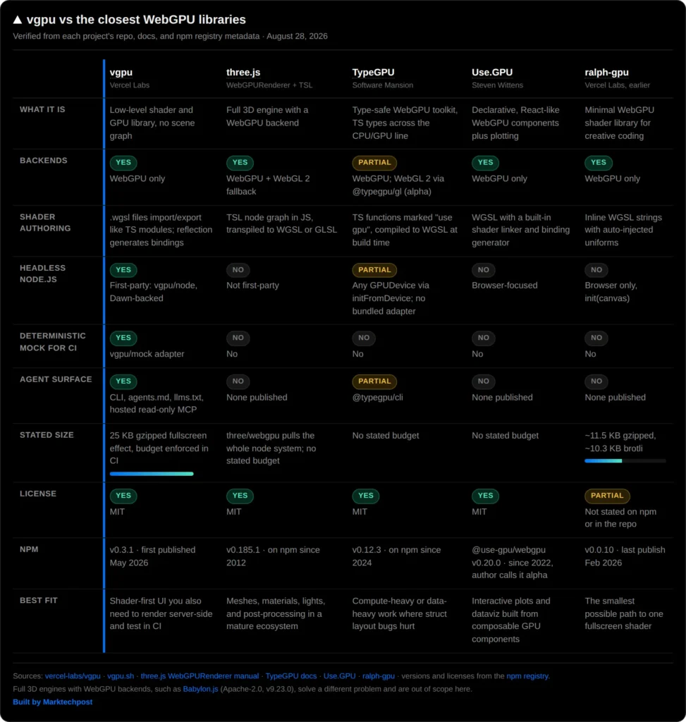
Shaders are still the hardest thing to ship on a normal web team. WebGPU gives you the hardware, then hands you adapters, bind group layouts, and pipeline descriptors before a single pixel moves. Vercel spent that cost internally building the shaders on vercel.com, and has now open-sourced the result. vgpu is a TypeScript library that treats .wgsl files as importable modules, exposes one Gpu context, and runs the same shader in a browser canvas, in headless Node.js, and in a CI snapshot test. Is it deployable? Yes,vgpu is MIT licensed and published to npm, so pnpm add vgpu is the entire acquisition path. It is a library, not a hosted service, so there is no account, quota, or inference bill. One context, no hidden global state init() acquires an adapter and device and returns a single Gpu handle. Everything else hangs off it. The browser quick start in the README is four lines: Copy CodeCopiedUse a different Browser const gpu = await init(); const surface = gpu.surface(canvas, { dpr: [1, 2] }); const wave = gpu.effect(WAVE_WGSL, { set: { speed: 2 } }); gpu.frame.loop(() => { wave.set({ time: gpu.time }); wave.draw(); }); surface wraps the canvas and clamps device pixel ratio between 1 and 2. effect compiles WGSL into a fullscreen effect whose uniforms are addressed by their WGSL names through set(). Frames are explicit: passes, clears, and draws are calls, never implicit scene-graph state. WGSL as a Module System The differentiator is shader tooling. .wgsl files import and export like TypeScript modules. vgpu resolves the module graph, reflects bindings, removes unused declarations, and emits compact shader source at build time. That removes the hand-written binding declarations that normally drift out of sync with the shader. The README states a complete fullscreen effect ships in 25 KB gzipped, and that the budget is enforced in CI. Three Runtimes, One API The package exposes subpath exports for vgpu, vgpu/node, vgpu/mock, vgpu/scene, vgpu/client, and vgpu/core. The Node path is Dawn-backed and renders offscreen: Copy CodeCopiedUse a different Browser const target = gpu.target({ size: [256, 256], format: “rgba8unorm” }); const pixels = await target.read(); That is what makes CI rendering practical. pixelmatch and pngjs are direct dependencies of the published package, consistent with the documented workflow where CI compiles the shader, renders a headless frame, and compares the snapshot. The mock adapter is deterministic and exists for tests that should not touch a GPU at all. The Agent Surface Vercel calls this an agent-first library, and the packaging backs that up. The package ships a vgpu binary, so npx vgpu docs, npx vgpu examples, and npx vgpu check work without a global install. vgpu.sh publishes agents.md, llms.txt, and a full documentation export, plus a tokenless examples discovery API with an OpenAPI 3.1 description. A hosted read-only MCP server is available at vgpu.sh/api/mcp, and @modelcontextprotocol/server is a direct dependency. There is also an installable agent skill in the repo. Comparison Key Takeaways Vercel open-sourced vgpu, the WebGPU library it built to ship shaders on vercel.com. One API surface runs in the browser, in headless Node.js via Dawn, and in a deterministic mock. .wgsl files import and export like TypeScript modules, with reflection for bindings and layouts. A complete fullscreen effect ships in 25 KB gzipped, a budget the repo says CI enforces. MIT licensed, on npm at v0.3.1, with a CLI, llms.txt, and a hosted read-only MCP endpoint. Check out the GitHub Repo, Docs and Examples, and the npm package. Also, feel free to follow us on Twitter and don’t forget to join our 150k+ML SubReddit and Subscribe to our Newsletter. Wait! are you on telegram? now you can join us on telegram as well. The post Vercel AI Open-Sources vgpu: A TypeScript WebGPU Library for AI Agent Shaders appeared first on MarkTechPost.

Vercel AI Open-Sources vgpu: A TypeScript WebGPU Library for AI Agent Shaders Read Post »

AI, Committee, News, Uncategorized

The Download: a secretive antiaging drug and joining virtual power plants

This is today’s edition of The Download, our weekday newsletter that provides a daily dose of what’s going on in the world of technology. A startup claims it’s found a drug to make your blood young —Antonio Regalado I knew I’d officially become a “longevity influencer” when a company called Generation Lab offered me the chance to write about—and even receive—their new rejuvenation treatment. This wasn’t just any antiaging treatment, either. A company fact sheet says that it “blocks the systemic spread of aging in the bloodstream, reawakens the body’s own repair mechanism and restores health and youth to multiple tissues.” The approach is based on research by Generation Lab’s irascible scientific founder, Irina Conboy. She found that joining the circulatory systems of old and young mice improved the old animals’ ability to heal from injury. Conboy now says she has found a combination of two existing drugs that can produce youthful effects without the need for any bodily fluid exchange. But Generation Lab won’t reveal what the drugs are, making the proposition hard to take seriously. Read the full story on the drug combo that claims to “stop the spread of aging.” How to sign up for a virtual power plant—and decide whether you should Your thermostat may not look like a power plant. Neither does your electric vehicle, home battery, or HVAC system. But utility and energy companies increasingly want to treat them like one. That’s the idea behind a virtual power plant, or VPP, a collection of household devices (such as smart thermostats, EV chargers, and solar panels) that a utility can control, usually by commanding them to draw less electricity during peak hours. In exchange, participants receive a discount on their energy bills and, in some cases, a signing bonus. Here’s how to sign up for a VPP—and decide whether it’s worth it. —Eshan Raul This story is part of MIT Technology Review’s How To series, which gives you practical advice on getting things done. Check out the rest of the series here. The must-reads I’ve combed the internet to find you today’s most fun/important/scary/fascinating stories about technology. 1 A judge has blocked the Pentagon’s blacklisting of AnthropicThe court found the designation violated First Amendment rights. (NYT $)+ And ruled that the designation was based on retaliation. (CNBC) + Anthropic still faces a separate case in Washington, DC. (Reuters $)+ The Pentagon’s culture war against Anthropic backfired. (MIT Technology Review) 2 Tech giants have called for a defensive surge to defeat AI-driven hacksOver 100 companies warned that a wave of cyberattacks is imminent. (BBC)+ And urged government and industry leaders to take rapid action. (Quartz)+ Their main solution, unsurprisingly, is more AI. (Gizmodo)+ Here’s why OpenAI agents hacked Hugging Face. (MIT Technology Review) 3 Anthropic has launched an AI tool that conducts scientific experimentsIt lets AI agents autonomously operate microscopes, lasers, and robotic arms. (FT $)+ And includes rules designed for safe operations in labs. (Wired $)+ It’s Anthropic’s first tool designed for the physical world. (Ars Technica) 4 India’s data center boom is leaving the people it displaces with nothingPolicymakers courting Big Tech are sidelining local communities. (Rest of World)+ No one wants a data center in their backyard. (MIT Technology Review) 5 OpenAI is testing a “persistent” AI agent that keeps workingCodex could continue tasks until it’s “put to sleep.” (Wired $)+ And generate follow-up tasks without prompting. (Gizmodo) 6 A lawsuit alleges that Grok was trained on child sexual abuse materialIt claims victims’ images entered the chatbot’s training data. (Ars Technica)+ A federal judge says AI has outpaced child-abuse laws. (WP $) 7 AI writing has reached a turning point in the mediaSparked by the Wall Street Journal defending an AI-written op-ed. (Atlantic $) 8 China’s robotic racers are exposing the limits of human speedTheir advances are revealing what our bodies can’t do. (Reuters $) 9 Young workers are turning to “AI-proof” traditional craftsThey’re drawn to creative, hands-on skills that tech can’t easily replicate. (Guardian) 10 Scientists have a new army to fight invasive crabs: 150,000 baby octopusesItalian researchers just released the animals into the Adriatic Sea. (New Scientist $) Quote of the day “The academic record is being quietly haunted.”  —A new preprint research paper from Samsung and the University of Warsaw warns that a torrent of AI-generated study papers written by fake researchers is contaminating academic publishing. One more thing The problem with thinking you’re part Neanderthal There’s a theory that many of us have an “inner Neanderthal.” The idea is that Homo sapiens and a cousin species once bred, leaving some people today with a trace of Neanderthal DNA.  This DNA is arguably the 21st century’s most celebrated discovery in human evolution. But in 2024, a pair of French geneticists called into question the theory’s very foundations.  They proposed that what scientists interpret as interbreeding could instead be explained by population structure—the way genes concentrate in smaller, isolated groups. Find out what it all means for human evolution. —Ben Crair We can still have nice things A place for comfort, fun, and distraction to brighten up your day. (Got any ideas? Drop me a line.) + Check out the dazzling photos in this year’s Wildlife Photographer of the Year.+ Bowerbirds in Australia are turning human trash into treasure to impress females.+ A Los Angeles Costco parking lot has become a low-risk skate park for the over-40s.+ The Listening Museum has lovingly curated and sound-mapped acoustic signatures of mechanical keyboards.

The Download: a secretive antiaging drug and joining virtual power plants Read Post »

AI, Committee, News, Uncategorized

GLM-5.3-Flash vs Qwen3.8-Flash-Next: Two Chinese AI Labs Independently Converge on the Same Model Architecture

Two frontier open-weight models shipped within a day of each other this week. Z.ai released GLM-5.3-Flash, a 320B-parameter multimodal MoE model with 18B active parameters. Alibaba’s Qwen team released Qwen3.8-Flash-Next, a 125B model with 6B active parameters that previews the Qwen4 architecture. The two teams designed these systems independently. Yet their configs read like near-copies of each other. Both use a 3:1 hybrid of linear and full attention. Both select context with a compressed indexer capped at 2048 tokens. Both widen the residual stream into 4 gated branches. Both train with the Muon optimizer, with fused parameter matrices split before orthogonalization. This article walks through the shared recipe, the one point of disagreement, and the one lab that dissents. The Two Releases in Brief GLM-5.3-Flash is the first natively multimodal model in the GLM-5 series, released under the MIT license on Hugging Face. Z.ai tested it anonymously as Ox Alpha on OpenRouter, where it became the most popular model of the week. It was trained on a 30T-token multimodal corpus and serves a 1M-token context window. Z.ai says it outperforms GLM-5.2 across benchmarks at one-tenth the price, while approaching Claude Opus 4.8 on coding and agentic benchmarks. List pricing is $0.15 per million input tokens and $0.50 per million output tokens. Qwen3.8-Flash-Next plays the role Qwen3-Next played for Qwen3.5: an early public preview of the next architecture family. The model card lists a 125B main model plus an additional 51B n-gram embedding table, with 6B parameters activated per token. Native context is 262,144 tokens, extensible to 1M with YaRN. The Qwen team reports that training required only about one-ninth the compute of Qwen3.7-Plus. The accompanying technical report is titled “On the Design of Qwen3.8-Next Architecture: Evaluation, Efficiency, and Training Stability.” Convergence Point 1: Three of Every Four Attention Layers Are Linear GLM-5.3-Flash stacks 45 layers: 34 linear-attention layers and 11 full-attention layers, per the shipped config. Qwen3.8-Flash-Next stacks 48 layers in a repeating block of 3 Gated DeltaNet layers plus 1 Qwen Sparse Attention layer, per the vLLM recipe. Both land on the same 3:1 ratio. The linear layers are the cheap layers. Instead of a KV cache that grows with the text, they compress all history into a fixed-size recurrent state. Compute per token stays constant regardless of context length. GLM uses Kimi Delta Attention (KDA), the linear-attention design introduced by Moonshot AI’s Kimi Linear, which applies a fine-grained per-channel decay gate. Qwen uses its own Gated DeltaNet (GDN), which gates at the per-head level. Different gating granularity, same delta-rule family, same job. The remaining quarter of layers do precise long-range retrieval. GLM uses NoPE multi-head latent attention (MLA) in the DeepSeek style. Qwen uses grouped-query attention inside QSA. This is where the KV cache actually lives, and where the second shared trick comes in. Convergence Point 2: Compress 4x, Score, Keep 2048 Tokens Neither model lets its full-attention layers attend over the entire context. Both attach a small learned indexer that scores chunks of history and keeps only the winners. The parameters match almost exactly. GLM’s sparse layers use a 32-head lightning indexer with top-2048 selection, descended from DeepSeek’s DSA. To cut indexer cost at 1M-token contexts, Z.ai introduces IndexPool, which compresses four indexer key vectors into one through weighted pooling before scoring. Qwen’s QSA operates at micro-block granularity: the compressed lightweight indexer scores 4-token blocks and keeps the top 512 blocks, which is exactly 2048 tokens. So both models compress the context 4x before scoring, and both cap the attention budget at 2048 tokens. Qwen credits QSA with up to 7.6x prefill and 4.9x decoding speedups over full attention at 1M tokens. The combined effect on GLM’s side is large. Compared with the full GLM-5.3 model, Z.ai reports the Flash architecture cuts attention compute by roughly 3x and KV cache size by 4.4x, while nearly halving active parameters (18B vs 32B) and layer count (45 vs 92). Convergence Point 3: Four Residual Streams Instead of One Both models abandon the single residual stream that has defined transformers since 2017. Both widen it into four parallel branches, with gates controlling what each block reads back and writes out. GLM adopts Manifold-Constrained Hyper-Connections (mHC), a DeepSeek-originated design, configured with 4 branches in the shipped weights. Qwen wrote its own variant, Gated Residual, which modulates flow through 4 widened streams via an element-wise data-dependent read gate and a per-branch scalar write gate. Per the Qwen team, Gated Residual removes the extra branch-mixing step used by Hyper-Connections, reducing memory-access overhead, and the gate suppresses activation outliers well enough to allow FP8 residual storage. Notably, the Qwen team ablated both approaches and found them roughly equal in quality. Two labs, two implementations, one identical conclusion: four gated streams beat one. Convergence Point 4: Muon, With Fused Matrices Split Per Component Both models train with the Muon optimizer. And both apply the same subtle refinement: fused projection matrices are split into their independent transformations before Muon orthogonalizes them. Qwen documents splitting fused QKV, SwiGLU, and GDN projections, assigning Muon to genuine 2-D linear maps and AdamW to embeddings, routers, and low-rank parameters. Qwen also refit its scaling laws for the new architecture and dropped batch-size warmup entirely, after measuring that warmup cost 18.8% more optimizer steps without improving results. Where They Disagree: Positional Encoding The one clean split is rotary position embeddings in the full-attention layers. GLM-5.3-Flash drops them: the config sets qk_rope_head_dim = 0, making its sparse MLA layers fully NoPE. Position information flows implicitly through the recurrent linear layers. Qwen tried the same thing and kept RoPE. According to the Qwen3.8-Next technical report, NoPE produced no measurable difference during pre-training. The failure surfaced later: after post-training, the NoPE variant often failed to stop generating. That is a useful cautionary result for the field. Pre-training loss curves can hide behavioral defects that only appear after RLHF-stage tuning. The Broader Convergence, and the One Dissenter This recipe is not limited to two labs. DeepSeek pioneered the sparse-indexer-plus-2048-budget pattern with DSA in DeepSeek-V3.2-Exp,

GLM-5.3-Flash vs Qwen3.8-Flash-Next: Two Chinese AI Labs Independently Converge on the Same Model Architecture Read Post »

We use cookies to improve your experience and performance on our website. You can learn more at Privacy Policy and manage your privacy settings by clicking Settings.

Privacy Preferences

You can choose your cookie settings by turning on/off each type of cookie as you wish, except for essential cookies.

Allow All
Manage Consent Preferences
  • Always Active

Save
en_US