YouZum

Committee

AI, Committee, News, Uncategorized

What Anthropic’s latest AI discovery does—and doesn’t—show

This story originally appeared in The Algorithm, our weekly newsletter on AI. To get stories like this in your inbox first, sign up here. Anthropic—currently the world’s most valuable AI company, with a nearly $1 trillion valuation—has a reputation for publishing strange and heady research. It’s looking into whether AI models can feel pain, for example, and will sometimes cut off chatbot conversations if it suspects users are “abusing” the model.  One niche that Anthropic spends more time and money on than other AI companies is called mechanistic interpretability, which means looking inside the complex math of an AI model to learn why it comes up with one particular output and not another. It’s complicated stuff; there are millions of data points that might contribute to any result, and wading through them can look more like word salad than anything useful. It’s also controversial. Describing AI models with terms borrowed from psychology and neuroscience can make their behavior seem more sophisticated than we might otherwise judge it to be. That’s why, when Anthropic announced last week that it had found a new window into its models’ “internal thoughts” as they reason through answers, there was one colleague I had to talk to. Senior editor Will Douglas Heaven, aside from having a PhD in computer science, has spent a lot of time digging into what we can say about how AI models work. I spoke with him about what we should take from Anthropic’s new (and predictably quirky) research. What did Anthropic learn here, exactly? Anthropic has been trying to understand how large language models (LLMs) work for a few years now. Anthropic isn’t the only one looking at this, but I think the company has made it part of its core mission more than most. Anthropic’s CEO, Dario Amodei, has said we won’t be able to control LLMs fully unless we learn more about how they work.  So this new research is very much in that context. It goes deeper into the weird mechanisms inside LLMs than ever before. What Anthropic learned was that LLMs have a space inside them—which Anthropic calls the J-space—filled with words that don’t appear in their output but that seem to influence the way they puzzle through problems. All this was hidden until Anthropic developed a new technique to probe its model Claude, so it’s a genuine discovery.  Sometimes these words keep track of where the LLM has got to in a particular task, sometimes they look more like flashes of recognition (for example, “protein” might pop up when you give an LLM only the letters of a protein sequence), and sometimes they represent a kind of internal commentary on the model’s decision-making. In my favorite example, Claude decided to cheat on a coding test when the word “panic” appeared. Anthropic also found that LLMs are able to describe and manipulate the words in this space. So somehow they seem to be making use of it.  Let’s step back for a second. I don’t think of large language models as simple, but they’re also not magic. There’s a bunch of math that learns relationships between words, right? So why is it so hard to “peer” into an LLM to know what’s going on? Yeah, they’re not magic! I think the fact we don’t fully understand them plays into the mythmaking. And it’s worth noting that the whole narrative that Anthropic is leaning into here—that they’ve built this really mysterious technology, but don’t worry, because they’re also the ones to figure it out—very much fits with the company’s vibe. [See how Anthropic warned that its new models were so good at coding they posed a global cybersecurity risk, only for the US government to shut them down shortly thereafter.] So yes: LLMs are just math. And yet it’s vastly complex math. Not only are today’s LLMs made out of hundreds of billions of numbers, but running them triggers a cascade of millions and millions of calculations. I wrote last year that if you printed out even a medium-size LLM on pieces of paper, it would cover a city the size of San Francisco.  It’s impossible to make sense of any of that math without specialist tools that highlight specific parts of an LLM at specific times. You need to know where to look and how to look. And building those tools requires understanding something of that complex math in the first place.  You’ve written elsewhere about this concept of studying LLMs the way one might study an organism’s brain. Is it fair to use “brain-like” terms when talking about how an LLM works? I don’t love using those kinds of terms. LLMs are not brains. Talking like this is misleading because it can suggest that LLMs are capable of more human-like things than they are or that we can make assumptions about how they might behave that we shouldn’t. The whole anthropomorphization thing is also tied up with a bunch of strong ideological positions about what this technology is and what it’s going to be.  But at the same time, we lack a good alternative vocabulary for talking about what these models are doing. I can understand why people reach for words like “think” and “understand” and “brain-like”—they’re convenient shorthand.  Anthropic compares this new space it found inside LLMs to the space that some neuroscientists think our brains use to keep track of conscious thoughts. I asked the company how seriously we should take that comparison and it said in a statement: “Drawing these analogies was helpful to us in designing our experiments, as they allowed us to make many non-obvious experimental predictions about the J-space that turned out to be true. At the same time, it’s important to note that there are some important differences between the J-space (and language models in general) and the human brain, so we don’t mean to claim there’s a perfect correspondence.”  What’s a problem in AI that this new concept of the J-space might be used to solve? Anthropic

What Anthropic’s latest AI discovery does—and doesn’t—show Read Post »

AI, Committee, News, Uncategorized

How to Build a T4-Friendly Autonomous Data Science Agent with DeepAnalyze-8B, Sandboxed Code Execution, and Iterative Analysis

In this tutorial, we build an autonomous data science agent around DeepAnalyze-8B and run it. We begin by preparing a stable runtime, installing the required machine-learning dependencies, and loading the DeepAnalyze tokenizer and model in 4-bit mode to keep the workflow practical on limited GPU memory. We then create a sandboxed execution environment that allows the model to generate Python code, execute it safely, observe the results, and continue its analysis in an agentic loop. By the end of the workflow, we give the agent a realistic multi-file e-commerce workspace and let it clean, join, analyze, visualize, and summarize the data as a structured analyst-grade report. Installing DeepAnalyze-8B Runtime Dependencies Copy CodeCopiedUse a different Browser import os, sys, subprocess os.environ[“MPLBACKEND”] = “Agg” def _pip(*args): subprocess.check_call([sys.executable, “-m”, “pip”, “install”, “-q”, *args]) _SETUP_FLAG = “/content/.da_ready” if not os.path.exists(_SETUP_FLAG): print(“Installing dependencies (one-time). The runtime will RESTART; ” “just re-run this cell afterwards.n”) _pip(“-U”, “transformers>=4.44”, “accelerate>=0.30”, “bitsandbytes>=0.43”) _pip(“sentencepiece”) _pip(“openpyxl”) _pip(“–force-reinstall”, “numpy==2.0.2”) open(_SETUP_FLAG, “w”).close() print(“nDependencies ready. Restarting runtime now…”) os.kill(os.getpid(), 9) We start by preparing the Colab runtime with the required machine-learning dependencies for DeepAnalyze-8B. We install the transformer, acceleration, quantization, tokenizer, and spreadsheet libraries without disturbing the broader notebook workflow. We also pin NumPy and restart the runtime once to keep the environment clean and stable for the next execution. Loading DeepAnalyze-8B in 4-Bit Mode Copy CodeCopiedUse a different Browser import re, io, glob, time, signal, contextlib, warnings, traceback from threading import Thread import numpy as np, pandas as pd import torch from transformers import (AutoModelForCausalLM, AutoTokenizer, BitsAndBytesConfig, TextIteratorStreamer) warnings.filterwarnings(“ignore”) MODEL_ID = “RUC-DataLab/DeepAnalyze-8B” USE_4BIT = True COMPUTE_DT = torch.float16 assert torch.cuda.is_available(), ( “No GPU detected. In Colab: Runtime -> Change runtime type -> GPU.”) print(“GPU:”, torch.cuda.get_device_name(0), “| NumPy:”, np.__version__) print(“nLoading tokenizer & model (first run downloads ~16GB, be patient)…”) tok = AutoTokenizer.from_pretrained(MODEL_ID, trust_remote_code=True) if tok.pad_token_id is None: tok.pad_token = tok.eos_token bnb = BitsAndBytesConfig( load_in_4bit=True, bnb_4bit_quant_type=”nf4″, bnb_4bit_compute_dtype=COMPUTE_DT, bnb_4bit_use_double_quant=True, ) if USE_4BIT else None model = AutoModelForCausalLM.from_pretrained( MODEL_ID, quantization_config=bnb, device_map=”auto”, torch_dtype=COMPUTE_DT, low_cpu_mem_usage=True, trust_remote_code=True, ) model.eval() print(“Model loaded. VRAM used: %.1f GB” % (torch.cuda.memory_allocated()/1e9)) We import the main libraries, configure the DeepAnalyze-8B model, and verify that a GPU is available in Colab. We load the tokenizer and prepare 4-bit quantization so the model can fit more comfortably on a T4 GPU. We then load the model in evaluation mode and confirm GPU memory usage before moving on to the agent logic. Building the Sandboxed Code Executor Copy CodeCopiedUse a different Browser class CodeSandbox: def __init__(self, timeout=120, max_chars=6000): self.ns = {“__name__”: “__main__”} self.timeout, self.max_chars = timeout, max_chars def _run(self, code): with contextlib.redirect_stdout(io.StringIO()) as out, contextlib.redirect_stderr(io.StringIO()) as err: exec(compile(code, “<cell>”, “exec”), self.ns) return out.getvalue() + err.getvalue() def execute(self, code): def _handler(signum, frame): raise TimeoutError(f”Execution exceeded {self.timeout}s”) prev = signal.signal(signal.SIGALRM, _handler) signal.alarm(self.timeout) try: out = self._run(code) result = out if out.strip() else “[Executed successfully, no stdout]” except Exception as e: tb = traceback.format_exc().splitlines() loc = next((l.strip() for l in tb if ‘”<cell>”‘ in l), “”) result = f”[Error]n{loc}n{type(e).__name__}: {e}”.strip() finally: signal.alarm(0) signal.signal(signal.SIGALRM, prev) if len(result) > self.max_chars: result = result[:self.max_chars] + “n…[output truncated]…” return result We define a sandboxed code executor that gives the agent a persistent Python namespace for running generated code. We capture standard output and error streams so that every execution result can be passed back into the reasoning loop. We also enforce a timeout and truncate long outputs to keep the autonomous workflow controlled and readable. Implementing the DeepAnalyze Agentic Loop Copy CodeCopiedUse a different Browser class DeepAnalyzeAgent: def __init__(self, model, tok, temperature=0.5, top_p=0.95): self.model, self.tok = model, tok self.temperature, self.top_p = temperature, top_p def _stream_generate(self, context, max_new_tokens): inputs = self.tok(context, return_tensors=”pt”, add_special_tokens=False).to(self.model.device) streamer = TextIteratorStreamer(self.tok, skip_prompt=True, skip_special_tokens=False) kwargs = dict( **inputs, max_new_tokens=max_new_tokens, do_sample=True, temperature=self.temperature, top_p=self.top_p, stop_strings=[“</Code>”], tokenizer=self.tok, streamer=streamer, pad_token_id=self.tok.pad_token_id, eos_token_id=self.tok.eos_token_id, ) Thread(target=self.model.generate, kwargs=kwargs).start() pieces = [] for chunk in streamer: pieces.append(chunk); print(chunk, end=””, flush=True) return “”.join(pieces) @staticmethod def _extract_code(delta): if “<Code>” in delta and “</Code>” not in delta: delta += “</Code>” m = re.search(r”<Code>(.*?)</Code>”, delta, re.DOTALL) if not m: return None code = m.group(1).strip() fenced = re.search(r”“`(?:python)?(.*?)“`”, code, re.DOTALL) return (fenced.group(1) if fenced else code).strip() def run(self, instruction, workspace, max_rounds=12, max_new_tokens=3072, exec_timeout=120): prompt = build_prompt(instruction, workspace) prefix = self.tok.apply_chat_template( [{“role”: “user”, “content”: prompt}], tokenize=False, add_generation_prompt=True) sandbox = CodeSandbox(timeout=exec_timeout) full, trace = prefix, [] cwd0 = os.getcwd(); os.chdir(workspace) try: for r in range(max_rounds): print(f”nn{‘=’*70}n ROUND {r+1}n{‘=’*70}”) delta = self._stream_generate(full, max_new_tokens) full += delta trace.append((“model”, delta)) if “<Answer>” in delta: print(“nn[Agent finished: <Answer> produced]”); break code = self._extract_code(delta) if code is None: print(“nn[Agent stopped: no further action]”); break output = sandbox.execute(code) print(f”nn— <Execute> —n{output}n— </Execute> —“) full += f”n<Execute>n{output}n</Execute>n” trace.append((“execute”, output)) else: print(f”nn[Reached max_rounds={max_rounds}]”) finally: os.chdir(cwd0) answer = “” if “<Answer>” in full: answer = full.split(“<Answer>”)[-1] answer = re.sub(r”</?Answer>”, “”, answer) answer = re.sub(r”<[||][^>]*?[||]>”, “”, answer).strip() return {“full”: full, “trace”: trace, “answer”: answer} We implement the DeepAnalyze agent loop, which streams model outputs, extracts the generated code, and executes it step by step. We allow the model to alternate between reasoning, coding, execution feedback, and final answering through special action tags. We maintain the full conversation trace so the agent can refine its analysis based on previous outputs and execution results. Running the E-Commerce Analysis Workspace Copy CodeCopiedUse a different Browser def _hsize(nbytes): for u in [“B”, “KB”, “MB”, “GB”]: if nbytes < 1024: return f”{nbytes:.1f}{u}” nbytes /= 1024 return f”{nbytes:.1f}TB” def build_prompt(instruction, workspace): exts = (“.csv”, “.xlsx”, “.xls”, “.json”, “.xml”, “.yaml”, “.yml”, “.txt”, “.md”, “.tsv”, “.db”, “.sqlite”) files = sorted(f for f in os.listdir(workspace) if f.lower().endswith(exts)) lines = [f’File {i+1}: {{“name”: “{f}”, “size”: “‘ f'{_hsize(os.path.getsize(os.path.join(workspace, f)))}”}}’ for i, f in enumerate(files)] return f”# Instructionn{instruction}nn# Datan” + “n”.join(lines) WORKSPACE = “/content/da_workspace” os.makedirs(WORKSPACE, exist_ok=True) rng = np.random.default_rng(42); N = 2500 categories = [“Electronics”, “Home”, “Fashion”, “Books”, “Toys”] dates = pd.to_datetime(“2024-01-01″) + pd.to_timedelta(rng.integers(0, 365, N), unit=”D”) tx = pd.DataFrame({ “order_id”: np.arange(100000, 100000 + N), “date”: dates, “customer_id”: rng.integers(1, 601, N), “category”: rng.choice(categories, N, p=[.3, .2, .25, .15, .1]), “region”: rng.choice([“North”, “South”, “East”, “West”], N), “quantity”: rng.integers(1, 6, N), “unit_price”: np.round(rng.gamma(3, 12, N) + 5, 2), “discount”: np.round(rng.choice([0, .05, .1, .15, .2], N), 2), }) tx[“revenue”] = np.round(tx.quantity *

How to Build a T4-Friendly Autonomous Data Science Agent with DeepAnalyze-8B, Sandboxed Code Execution, and Iterative Analysis Read Post »

AI, Committee, News, Uncategorized

Kyutai Releases MuScriptor: An Open-Weight Decoder-Only Transformer for Multi-Instrument Music Transcription to MIDI

Automatic Music Transcription (AMT) converts an audio recording into symbolic notes, usually MIDI. Single-instrument transcription already works reasonably well. However, transcribing a full multi-instrument mix stays difficult. Kyutai and Mirelo team now release MuScriptor to close that gap. It is an open-weight model trained on real, multi-instrument recordings across many genres. This article explains how MuScriptor works, what the benchmarks show, and how to run it. What is MuScriptor? At its core, MuScriptor is a decoder-only Transformer for music transcription. First, it reads a mel-spectrogram of a short audio segment. Then it autoregressively predicts MIDI-like tokens for pitch, timing, and instrument. In effect, transcription becomes a language-modeling task, following the MT3 tokenization scheme. The release ships three weight variants on Hugging Face. Their sizes are small (103M), medium (307M, default), and large (1.4B). The inference code uses the MIT license. The weights use CC BY-NC 4.0, so commercial use is restricted. How the Three-Stage Pipeline Works MuScriptor’s main idea is data, not architecture. Accordingly, training moves through three stages, and each builds on the last. Pre-training uses D<sub>Synth</sub>, roughly 1.45M MIDI files. An on-the-fly pipeline synthesizes them during training. Augmentations include pitch shifting, tempo changes, velocity adjustment, and instrument randomization. Over 250 soundfonts plus random detuning yield near-infinite audio realizations. Fine-tuning uses D<sub>Real</sub>, an internal set of 170,000 recordings. Together they total more than 11,000 hours with aligned note annotations. Most alignments come from audio-symbolic synchronization using interpolation and dynamic time warping. Poor pairs are filtered by warping distance and a maximum time-dilation factor. Reinforcement learning post-training uses D<sub>RL</sub>, 300 manually verified tracks. The team applies a GRPO-like method combining REINFORCE with group-relative advantage normalization. The reward sums three F-scores: onset, frame, and offset. As a result, the model learns to favor cleaner transcriptions. Transcribe</button> </div> </div> <div class=”rollwrap”> <svg class=”roll” id=”roll” viewBox=”0 0 720 300″ preserveAspectRatio=”xMidYMid meet” role=”img” aria-label=”Piano roll transcription”></svg> </div> <div class=”legend”> <span><i style=”background:#2563EB”></i>True positive (detected)</span> <span><i style=”background:#16A34A”></i>False negative (missed)</span> <span><i style=”background:#DC2626″></i>False positive (wrong)</span> </div> <div class=”grid”> <div class=”metrics”> <div class=”metric”> <small>Onset F1</small> <div class=”val” id=”mOnset”>—</div> <div class=”baseline” id=”bOnset”></div> <div class=”metricbar”><i id=”barOnset”></i></div> </div> <div class=”metric”> <small>Multi F1</small> <div class=”val” id=”mMulti”>—</div> <div class=”baseline” id=”bMulti”></div> <div class=”metricbar”><i id=”barMulti”></i></div> </div> </div> <div class=”stream” id=”stream”> <div class=”h”>Event stream · model.transcribe()</div> <div class=”ln” style=”opacity:.6″>Press Transcribe to stream note events…</div> </div> </div> <p class=”note” id=”stageNote”></p> </div> <div class=”foot”> <span>Note pattern is illustrative. F1 scores are real, from the MuScriptor paper (1.3B model on D<sub>Test</sub>).</span> <span>Built by <b>Marktechpost</b></span> </div> </div> <script> (function(){ var SVG=”http://www.w3.org/2000/svg”; var roll=document.getElementById(“roll”); var W=720,H=300,PADL=64,PADR=14,PADT=14,PADB=26; var DUR=10; // seconds shown var rows=[ {name:”Drums”,inst:”drums”,y:0}, {name:”E-Bass”,inst:”e_bass”,y:1}, {name:”Dist. E-Gtr”,inst:”distorted_e_guitar”,y:2}, {name:”Ac. Piano”,inst:”acoustic_piano”,y:3}, {name:”Voice”,inst:”voice”,y:4}, {name:”Strings”,inst:”string_ensemble”,y:5} ]; var NR=rows.length; var rowH=(H-PADT-PADB)/NR; function tx(t){return PADL+(t/DUR)*(W-PADL-PADR);} function ry(r){return PADT+r*rowH;} // Illustrative ground-truth notes: [row, start, dur, rank(0=easy..1=hard)] var GT=[ [0,0.3,0.18,0.1],[0,0.8,0.18,0.15],[0,1.3,0.18,0.2],[0,1.8,0.18,0.1],[0,2.4,0.18,0.25],[0,3.0,0.18,0.2],[0,3.6,0.18,0.3],[0,4.2,0.18,0.2],[0,4.9,0.18,0.4],[0,5.5,0.18,0.3],[0,6.2,0.18,0.5],[0,6.9,0.18,0.4],[0,7.6,0.18,0.6],[0,8.3,0.18,0.5],[0,9.0,0.18,0.7], [1,0.4,0.8,0.2],[1,1.6,0.8,0.25],[1,3.0,0.9,0.35],[1,4.4,0.8,0.4],[1,5.8,0.9,0.5],[1,7.2,0.9,0.6],[1,8.6,0.9,0.7], [2,1.0,1.1,0.45],[2,2.6,1.0,0.55],[2,4.2,1.2,0.6],[2,6.0,1.1,0.7],[2,7.8,1.1,0.8], [3,0.6,0.7,0.3],[3,1.7,0.6,0.35],[3,2.9,0.7,0.4],[3,4.1,0.6,0.5],[3,5.3,0.7,0.55],[3,6.6,0.6,0.65],[3,8.0,0.8,0.75], [4,2.0,1.4,0.5],[4,4.0,1.5,0.6],[4,6.3,1.4,0.72],[4,8.4,1.2,0.85], [5,1.2,1.8,0.55],[5,3.6,1.9,0.68],[5,6.0,1.9,0.8],[5,8.2,1.6,0.9] ]; // Illustrative false positives available: [row,start,dur,rank] var FPS=[ [0,2.1,0.16,0.9],[0,5.9,0.16,0.7],[0,7.9,0.16,0.85], [1,2.4,0.6,0.8],[1,6.6,0.7,0.9], [2,3.7,0.9,0.85],[2,8.9,0.9,0.95], [3,3.5,0.5,0.9],[3,7.3,0.6,0.8], [4,3.5,0.9,0.9],[4,7.7,0.8,0.95], [5,5.1,1.2,0.88],[5,9.2,0.9,0.97] ]; // Real numbers from the paper (1.3B, DTest). recall/fpRate are illustrative thresholds. var STAGES={ synth:{onset:34.5,multi:16.2,onBase:26.1,recall:0.42,fp:0.85, note:”Trained only on synthetic MIDI. It finds coarse pitch activity, but misses many onsets and mislabels instruments.”}, real:{onset:54.4,multi:41.6,onBase:52.5,recall:0.78,fp:0.35, note:”Fine-tuning on 170k real recordings lifts every metric by roughly 20 points over synthetic-only training.”}, rl:{onset:60.4,multi:48.2,onBase:60.4,recall:0.90,fp:0.12, note:”GRPO-style RL post-training on 300 verified tracks reduces false negatives and sharpens onset timing.”} }; var current=”rl”, cond=true, playing=false, playhead=0, raf=null, streamed={}; function selectedRows(){ if(!cond) return rows.map(function(r){return r.y;}); // conditioning example: focus on the core rhythm section + piano return [0,1,2,3]; } function classify(stage){ var s=STAGES[stage]; var tp=[],fn=[],fp=[]; var sel=selectedRows(); GT.forEach(function(n){ if(cond && sel.indexOf(n[0])===-1) return; // hidden by conditioning var boost=cond?0.08:0; // conditioning nudges recall up (illustrative) if(n[3] <= s.recall+boost) tp.push(n); else fn.push(n); }); FPS.forEach(function(n){ if(cond && sel.indexOf(n[0])===-1) return; var fpr=cond?s.fp*0.7:s.fp; // conditioning trims spurious notes if(n[3] > (1-fpr)) fp.push(n); }); return {tp:tp,fn:fn,fp:fp}; } function el(tag,attrs){var e=document.createElementNS(SVG,tag);for(var k in attrs)e.setAttribute(k,attrs[k]);return e;} function drawGrid(){ while(roll.firstChild) roll.removeChild(roll.firstChild); var sel=selectedRows(); for(var r=0;r<NR;r++){ var active=sel.indexOf(r)!==-1; roll.appendChild(el(“rect”,{x:PADL,y:ry(r),width:W-PADL-PADR,height:rowH, fill:(r%2? “#FAFBFD”:”#FFFFFF”),opacity:active?1:0.4})); roll.appendChild(el(“line”,{x1:PADL,y1:ry(r),x2:W-PADR,y2:ry(r),stroke:”#EFF1F5″,”stroke-width”:1})); var lbl=el(“text”,{x:PADL-8,y:ry(r)+rowH/2+4,”text-anchor”:”end”,”font-size”:11, fill:active?”#14161C”:”#B6BCC7″,”font-weight”:active?600:500,”font-family”:”Inter,sans-serif”}); lbl.textContent=rows[r].name; roll.appendChild(lbl); } // time gridlines every 2s (segment markers) for(var t=0;t<=DUR;t+=2){ roll.appendChild(el(“line”,{x1:tx(t),y1:PADT,x2:tx(t),y2:H-PADB,stroke:”#E7E9EE”,”stroke-width”:1,”stroke-dasharray”:”2 4″})); var tl=el(“text”,{x:tx(t),y:H-9,”text-anchor”:”middle”,”font-size”:10,fill:”#9AA1AE”,”font-family”:”Inter,sans-serif”}); tl.textContent=t+”s”; roll.appendChild(tl); } roll.appendChild(el(“line”,{x1:PADL,y1:H-PADB,x2:W-PADR,y2:H-PADB,stroke:”#E7E9EE”,”stroke-width”:1})); } var noteLayer,headLine; function render(reveal){ drawGrid(); var c=classify(current); noteLayer=el(“g”,{}); roll.appendChild(noteLayer); function bar(n,color,opacity){ var x=tx(n[1]),w=Math.max(6,tx(n[1]+n[2])-tx(n[1])); var y=ry(n[0])+rowH*0.28,h=rowH*0.44; var vis=(!reveal)|| (n[1]<=playhead); var rect=el(“rect”,{x:x,y:y,width:w,height:h,rx:3,fill:color,opacity:vis?opacity:0}); rect.style.transition=”opacity .18s”; noteLayer.appendChild(rect); } c.fn.forEach(function(n){bar(n,”#16A34A”,0.55);}); c.fp.forEach(function(n){bar(n,”#DC2626″,0.8);}); c.tp.forEach(function(n){bar(n,”#2563EB”,0.95);}); headLine=el(“line”,{x1:tx(playhead),y1:PADT,x2:tx(playhead),y2:H-PADB,stroke:”#5B9A00″,”stroke-width”:2,opacity:reveal?0.9:0}); roll.appendChild(headLine); postSize(); } function setMetrics(){ var s=STAGES[current]; animateNum(“mOnset”,s.onset); animateNum(“mMulti”,s.multi); document.getElementById(“bOnset”).textContent=”baseline YourMT3+ 32.5″; document.getElementById(“bMulti”).textContent=”baseline YourMT3+ 21.9″; document.getElementById(“barOnset”).style.width=s.onset+”%”; document.getElementById(“barMulti”).style.width=(s.multi/60*100)+”%”; document.getElementById(“stageNote”).textContent=s.note; } function animateNum(id,to){ var e=document.getElementById(id),from=parseFloat(e.textContent)||0,st=null,dur=550; function step(ts){if(!st)st=ts;var p=Math.min(1,(ts-st)/dur); e.textContent=(from+(to-from)*(1-Math.pow(1-p,3))).toFixed(1); if(p<1)requestAnimationFrame(step);} requestAnimationFrame(step); } // event stream var stream=document.getElementById(“stream”); function resetStream(){stream.innerHTML='<div class=”h”>Event stream · model.transcribe()</div>’;streamed={};} function pushEvent(n,kind){ var pitchNames=[“C2″,”G2″,”E3″,”C4″,”A4″,”D5”]; var line=document.createElement(“div”);line.className=”ln”; var p=pitchNames[n[0]]||”C4″;var inst=rows[n[0]].inst; if(kind===”start”){ line.innerHTML='<span class=”st”>NoteStart</span> t=<span class=”pi”>’+n[1].toFixed(2)+’s</span> pitch=<span class=”pi”>’+p+'</span> inst=<span class=”in”>’+inst+'</span>’; }else{ line.innerHTML='<span class=”en”>NoteEnd</span> t=<span class=”pi”>’+(n[1]+n[2]).toFixed(2)+’s</span> (‘+inst+’)’; } stream.appendChild(line);stream.scrollTop=stream.scrollHeight; } function play(){ if(playing)return; playing=true; var btn=document.getElementById(“playBtn”);btn.disabled=true;btn.textContent=”● Transcribing…”; playhead=0; resetStream(); var c=classify(current); var visible=c.tp.concat(c.fp).sort(function(a,b){return a[1]-b[1];}); render(true); var t0=null,SPEED=DUR/4200; // ms mapping function frame(ts){ if(!t0)t0=ts; playhead=Math.min(DUR,(ts-t0)*SPEED); // reveal notes + emit events visible.forEach(function(n,i){ var key=”s”+i; if(n[1]<=playhead && !streamed[key]){streamed[key]=1; var rects=noteLayer.querySelectorAll(“rect”); pushEvent(n,”start”); setTimeout((function(nn){return function(){pushEvent(nn,”end”);};})(n),120); } }); // update opacities Array.prototype.forEach.call(noteLayer.querySelectorAll(“rect”),function(r){}); render(true); if(playhead<DUR){raf=requestAnimationFrame(frame);} else{playing=false;btn.disabled=false;btn.textContent=” Transcribe again”; headLine.setAttribute(“opacity”,”0″);postSize();} } raf=requestAnimationFrame(frame); } // controls document.getElementById(“stages”).addEventListener(“click”,function(e){ var b=e.target.closest(“button”);if(!b)return; Array.prototype.forEach.call(this.children,function(c){c.classList.remove(“on”);}); b.classList.add(“on”);current=b.getAttribute(“data-s”); playhead=DUR;render(false);setMetrics();postSize(); }); document.getElementById(“condToggle”).addEventListener(“click”,function(){ cond=!cond;this.classList.toggle(“on”,cond); playhead=DUR;render(false);postSize(); }); document.getElementById(“playBtn”).addEventListener(“click”,play); // pipeline shimmer var pnodes=document.querySelectorAll(“#pipe .node”),pi=0; setInterval(function(){ pnodes.forEach(function(n){n.classList.remove(“hot”);}); pnodes[pi].classList.add(“hot”);pi=(pi+1)%pnodes.length; },900); // resize to parent (WordPress embed) function postSize(){ try{var h=document.body.offsetHeight+40; window.parent.postMessage({muscriptorHeight:h},”*”);}catch(e){} } window.addEventListener(“resize”,function(){render(false);postSize();}); // init playhead=DUR;render(false);setMetrics();setTimeout(postSize,60);setTimeout(postSize,400); })(); </script> </body> </html> “> Performance For evaluation, the research team use D<sub>Test</sub>, 372 held-out tracks with accurate annotations. They report instrument-agnostic metrics from the mir_eval library. Among them, Multi F1 is strictest, since it also requires the correct instrument. The table below traces each training stage against the YourMT3+ baseline, using the large (~1.3B) model. Model (D<sub>Test</sub>) Onset F1 Frame F1 Offset F1 Drums F1 Multi F1 YourMT3+ (baseline) 32.5 45.5 17.8 41.4 21.9 MuScriptor · D<sub>Synth</sub> 34.5 48.9 16.1 21.0 16.2 MuScriptor · D<sub>Synth</sub> + D<sub>Real</sub> 54.4 69.3 42.3 43.3 41.6 MuScriptor · D<sub>Synth</sub> + D<sub>Real</sub> + D<sub>RL</sub> 60.4 73.3 49.0 50.2 48.2 Clearly, every stage improves results, and real data matters most. Synthetic-only training reaches competitive frame F1 but weak onset and multi scores. Adding D<sub>Real</sub> then lifts all metrics by roughly 20 points. Finally, RL post-training reduces false negatives and sharpens onset timing.

Kyutai Releases MuScriptor: An Open-Weight Decoder-Only Transformer for Multi-Instrument Music Transcription to MIDI Read Post »

AI, Committee, News, Uncategorized

A Coding Guide to NVIDIA’s Tile-Based GPU Programming: From cuTile and Triton Kernels to Flash Attention

In this tutorial, we explore TileGym GPU programming by building a practical Colab workflow that runs across different hardware conditions. We begin by probing the available CUDA environment, checking whether NVIDIA cuTile runs directly, and falling back to Triton when standard Colab GPUs lack the required cuTile stack. Through this setup, we learn the core tile-programming idea: instead of writing code for one thread at a time, we operate on entire data tiles, load them into the kernel, compute on them efficiently, and store the results back. We use this model to implement vector addition, fused GELU, row-wise softmax, tiled matrix multiplication, and flash attention, while comparing each result against PyTorch for correctness and benchmarking. CUDA Environment Probe Copy CodeCopiedUse a different Browser import os, sys, math, time, textwrap def rule(t=””): print(“n” + “=” * 78) if t: print(t) print(“=” * 78) rule(“0. ENVIRONMENT PROBE”) try: import torch except ImportError: print(“Installing torch …”) os.system(f”{sys.executable} -m pip install -q torch”) import torch HAS_CUDA = torch.cuda.is_available() DEV = “cuda” if HAS_CUDA else “cpu” cc = (0, 0) if HAS_CUDA: cc = torch.cuda.get_device_capability() print(f”GPU : {torch.cuda.get_device_name(0)}”) print(f”Compute capability : {cc[0]}.{cc[1]}”) print(f”Torch CUDA runtime : {torch.version.cuda}”) print(f”Driver / torch : {torch.__version__}”) else: print(“No CUDA GPU found. In Colab: Runtime -> Change runtime type -> GPU (T4).”) print(“The tutorial will still run its correctness math on CPU where possible.”) CUTILE_HW_OK = HAS_CUDA and cc[0] >= 8 CUDA_MAJOR = int((torch.version.cuda or “0”).split(“.”)[0]) if HAS_CUDA else 0 CUTILE_TOOLKIT_OK = CUDA_MAJOR >= 13 rule(“1. ATTEMPTING REAL cuTile (NVIDIA CUDA Tile) BACKEND”) ct = None CUTILE_READY = False if CUTILE_HW_OK and CUTILE_TOOLKIT_OK: try: import cuda.tile as ct CUTILE_READY = True print(“cuda.tile is already importable.”) except Exception: print(“Installing cuda-tile[tileiras] (this can take a while)…”) os.system(f”{sys.executable} -m pip install -q ‘cuda-tile[tileiras]’ cupy-cuda13x”) try: import cuda.tile as ct CUTILE_READY = True except Exception as e: print(“cuTile import still failed:”, repr(e)) else: reasons = [] if not HAS_CUDA: reasons.append(“no CUDA GPU”) if HAS_CUDA and cc[0] < 8: reasons.append(f”compute capability {cc[0]}.{cc[1]} < 8.0 (Turing/T4 unsupported)”) if not CUTILE_TOOLKIT_OK: reasons.append(f”CUDA {torch.version.cuda} < 13.1 required by tileiras”) print(“Skipping real cuTile install because:”, “; “.join(reasons) + “.”) print(“This is expected on a standard Colab T4 — we fall back to Triton below,”) print(“which teaches the exact same tile-based programming model.”) if CUTILE_READY: BACKEND = “cutile” else: try: import triton, triton.language as tl BACKEND = “triton” if HAS_CUDA else “torch” except ImportError: if HAS_CUDA: print(“Installing triton …”) os.system(f”{sys.executable} -m pip install -q triton”) try: import triton, triton.language as tl BACKEND = “triton” except Exception: BACKEND = “torch” else: BACKEND = “torch” rule(f”ACTIVE EXECUTION BACKEND: {BACKEND.upper()}”) print({ “cutile”: “Running NVIDIA cuTile kernels on your Ampere+/CUDA13 GPU. Nice hardware!”, “triton”: “Running Triton tile kernels on your GPU (the standard Colab path).”, “torch”: “No usable GPU kernel backend; showing reference math on CPU only.”, }[BACKEND]) print(textwrap.dedent(“”” —————————————————————— SIMT (classic CUDA) | TILE model (cuTile / Triton) —————————————————————— You write code for ONE | You write code for ONE BLOCK that thread. You compute a global | owns a whole TILE (e.g. 1024 elems index, bounds-check it, and | or a 128×128 sub-matrix). You load touch a single element. | the tile, do math on the WHOLE tile, | store it. The compiler maps the tile C[i] = A[i] + B[i] | onto threads / tensor cores for you. —————————————————————— cuTile primitives: ct.bid(0), ct.load(…), ct.store(…), a @ b, ct.launch Triton primitives: tl.program_id, tl.load, tl.store, tl.dot, grid[…] Same idea, two spellings. Below, every kernel is shown in BOTH. “””)) CUTILE_SOURCE = { “vector_add”: ”’ import cuda.tile as ct @ct.kernel def vector_add(a, b, c, tile_size: ct.Constant[int]): pid = ct.bid(0) a_tile = ct.load(a, index=(pid,), shape=(tile_size,)) b_tile = ct.load(b, index=(pid,), shape=(tile_size,)) ct.store(c, index=(pid,), tile=a_tile + b_tile) ”’, “matmul”: ”’ import cuda.tile as ct @ct.kernel def matmul(A, B, C, K: ct.Constant[int], BM: ct.Constant[int], BN: ct.Constant[int], BK: ct.Constant[int]): m, n = ct.bid(0), ct.bid(1) acc = ct.zeros((BM, BN), dtype=ct.float32) for k in range(ct.cdiv(K, BK)): a = ct.load(A, index=(m, k), shape=(BM, BK)) b = ct.load(B, index=(k, n), shape=(BK, BN)) acc = a @ b + acc ct.store(C, index=(m, n), tile=acc) ”’} We begin by setting up the environment, importing the required libraries, and checking whether CUDA is available on the current runtime. We inspect the GPU capabilities, CUDA version, and PyTorch setup to determine whether the real cuTile backend is usable. We then select the active execution backend, explain the tile programming model, and store reference cuTile kernel source strings for comparison. Defining Triton Kernels Copy CodeCopiedUse a different Browser if BACKEND == “triton”: @triton.jit def _vadd_kernel(a_ptr, b_ptr, c_ptr, n, BLOCK: tl.constexpr): pid = tl.program_id(0) offs = pid * BLOCK + tl.arange(0, BLOCK) mask = offs < n a = tl.load(a_ptr + offs, mask=mask) b = tl.load(b_ptr + offs, mask=mask) tl.store(c_ptr + offs, a + b, mask=mask) @triton.jit def _fused_gelu_kernel(x_ptr, w_ptr, b_ptr, o_ptr, n, BLOCK: tl.constexpr): pid = tl.program_id(0) offs = pid * BLOCK + tl.arange(0, BLOCK) mask = offs < n x = tl.load(x_ptr + offs, mask=mask) w = tl.load(w_ptr + offs, mask=mask) b = tl.load(b_ptr + offs, mask=mask) h = x * w + b c = 0.7978845608028654 z = c * (h + 0.044715 * h * h * h) e = tl.exp(-2.0 * z) tanh = (1.0 – e) / (1.0 + e) g = 0.5 * h * (1.0 + tanh) tl.store(o_ptr + offs, g, mask=mask) @triton.jit def _softmax_kernel(x_ptr, o_ptr, stride, n_cols, BLOCK: tl.constexpr): row = tl.program_id(0) cols = tl.arange(0, BLOCK) mask = cols < n_cols ptr = x_ptr + row * stride + cols x = tl.load(ptr, mask=mask, other=-float(“inf”)) x = x – tl.max(x, axis=0) num = tl.exp(x) den = tl.sum(num, axis=0) tl.store(o_ptr + row * stride + cols, num / den, mask=mask) @triton.jit def _matmul_kernel(A, B, C, M, N, K, sam, sak, sbk, sbn, scm, scn, BM: tl.constexpr, BN: tl.constexpr, BK: tl.constexpr): pid_m = tl.program_id(0) pid_n = tl.program_id(1) offs_m = pid_m * BM + tl.arange(0, BM) offs_n = pid_n * BN + tl.arange(0, BN) offs_k = tl.arange(0, BK) a_ptr = A + offs_m[:, None] * sam + offs_k[None, :] * sak b_ptr

A Coding Guide to NVIDIA’s Tile-Based GPU Programming: From cuTile and Triton Kernels to Flash Attention Read Post »

AI, Committee, News, Uncategorized

Grounded Event Extraction from SEC 8-K Filings with a Fine-Grained Taxonomy

arXiv:2607.08346v1 Announce Type: new Abstract: Form 8-K filings are the primary channel through which U.S. public companies disclose material events, but the SEC item codes attached to them are coarse: a single item spans routine administrative changes and chief executive departures, and many of the most market-moving disclosures fall into a catch-all item. Large language models make fine-grained labelling feasible at corpus scale, but only if the labels can be traced to the source text and shown to be reliable. We present a two-stage system that tags 8-K disclosures against a three-tier taxonomy of 119 event types. The first stage constrains output to valid taxonomy entries and anchors every tag to a verbatim quote via fuzzy n-gram validation; the second re-grades each cited quote against the category definition to produce a quality score. Applying the system to 292,984 filings from 2022 to 2026 yields 601,088 grounded event tags, which we release. Over 5,125 stratified tags, an LLM judge finds precision rises monotonically with the quality score, from 12% to 96%, while unsupported tags fall from 8% to near zero. Ablation shows the score is calibrated only when assigned in a dedicated second pass. An event study on unsigned abnormal returns confirms, without any language model, that the taxonomy separates economically distinct events sharing an item code.

Grounded Event Extraction from SEC 8-K Filings with a Fine-Grained Taxonomy Read Post »

AI, Committee, News, Uncategorized

Can We Trust LLM’s Logic? Quantifying Uncertainty, Coherence, and Robustness via a Graph-Based Framework

arXiv:2607.08017v1 Announce Type: new Abstract: Large-Language Models (LLMs) can be prone to flawed and unfaithful reasoning that decoding strategies like Self-Consistency (SC) fail to detect as they evaluate only final-answer agreement while ignoring the logical validity of intermediate steps. This raises three fundamental questions: How can we reliably quantify uncertainty in LLM reasoning? Can semantic, structural, and causal awareness select more faithful reasoning compared to na”ive majority voting? and How robust is reasoning topology under adversarial conditions? To address these questions, we introduce GRAPHEVAL, a graph-based reasoning framework that re-frames uncertainty quantification (UQ) as a holistic reasoning fidelity problem. We propose a novel UQ metric, Graph Reasoning Coherence Score (GRCS), that quantifies semantic-structural consensus of the reasoning space and captures pathological mode collapse and confident hallucinations. We find that GRCS is the only metric that is consistently negatively correlated with reasoning faithfulness across both more capable and smaller models. Additionally, we introduce Graph Self-Consistency (GSC), a medoid-based decoding strategy that trades nominal accuracy for reasoning fidelity, exposing the degree to which SC is inflated by unfaithful lucky guesses in smaller models, while preserving or improving accuracy in more capable ones. Finally, through adversarial medoid ablation, we demonstrate that the GSC-selected path acts as a “load-bearing path” and forcing models away from it degrades reasoning faithfulness and, in targeted cases, causes drops in accuracy.

Can We Trust LLM’s Logic? Quantifying Uncertainty, Coherence, and Robustness via a Graph-Based Framework Read Post »

AI, Committee, News, Uncategorized

How to Leverage Synthetic Speech for LLM-Based ASR Systems?

arXiv:2606.29031v2 Announce Type: replace Abstract: In regulated domains such as banking and healthcare, where privacy constraints make real speech costly to collect and retain, synthetic speech from modern text-to-speech (TTS) is an appealing alternative for training automatic speech recognition (ASR) without exposing sensitive customer recordings. Yet a persistent distributional gap between synthetic and real data limits how far it can replace genuine recordings. Prior work largely treats this gap as a black box to be engineered around, but in our work, we instead examine its origin directly by probing a SLAM-ASR architecture. Then, we localise where its LLM backbone separates real from synthetic speech and find the discriminative signal concentrated in the early-to-middle layers, where temporal and prosodic perturbations disrupt it most. We further show that representation-level separability, help, but does not directly predict downstream ASR gains. On the other hand, convolving synthetic audio with room impulse responses (RIRs) narrows the gap not by making synthetic speech sound cleaner or more natural, but by reproducing the acoustic irregularities of real recordings. Translating these findings into the training procedure, by adding a layer-selection module combined with RIR augmentation matches a fully real-data baseline using only 25% of the real speech (13.6h) and surpasses it at all higher proportions.

How to Leverage Synthetic Speech for LLM-Based ASR Systems? Read Post »

AI, Committee, News, Uncategorized

UtterTune: LoRA-Based Target-Language Pronunciation Edit and Control in Multilingual Text-to-Speech

arXiv:2508.09767v3 Announce Type: replace-cross Abstract: We propose UtterTune, a lightweight method for adapting a multilingual text-to-speech (TTS) system built on a large language model (LLM). It improves control of pronunciation in the target language while preserving performance in the others. Although LLM architectures have enabled TTS models to achieve remarkable naturalness, accurately modeling grapheme-to-phoneme (G2P) mapping and prosody remains challenging, especially when the model omits an explicit G2P module and directly processes minimally encoded text (e.g., byte-pair encoding). UtterTune leverages low-rank adaptation to enable the control of segmental pronunciation and pitch accent at the phoneme level for Japanese speech, the target language in this paper, while maintaining naturalness and speaker similarity in a zero-shot setting. Objective and subjective evaluations confirm its effectiveness.

UtterTune: LoRA-Based Target-Language Pronunciation Edit and Control in Multilingual Text-to-Speech Read Post »

AI, Committee, News, Uncategorized

Ant Group’s Robbyant Unveils LingBot-VA 2.0: A Causal Video-Action Model Built Natively for Physical AI

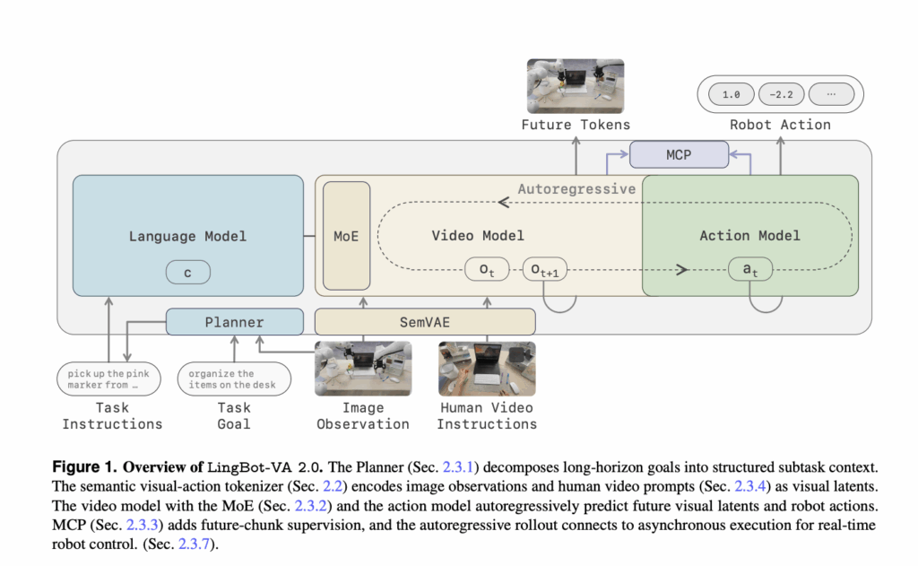
Robbyant, the embodied AI unit inside Ant Group, has released the LingBot-VA 2.0.The first embodied-native foundation model. It describes a video-action foundation model for generalist robot manipulation. The research team pretrains the whole stack for embodiment instead of fine-tuning a video generator. What is LingBot-VA 2.0? Most video-action models reuse two components built for digital content creation. One is a reconstruction-oriented VAE. The other is a bidirectional video-diffusion backbone, with an action module attached. This creates three limitations. Pixel-reconstruction latents preserve appearance but carry limited physical structure. Iterative denoising over video tokens is too slow for closed-loop control. Generic video objectives never teach how actions reshape the world. A fourth mismatch is structural. Backbones use bidirectional attention, while control unfolds strictly forward in time. LingBot VA Version 1.0 finetuned that stack into a causal model. Version 2.0 pretrains a causal DiT natively. https://github.com/Robbyant/lingbot-va/blob/main/LingBot_VA2_paper.pdf Version 1: The Semantic Visual-Action Tokenizer Building on that motivation, stage one replaces the compression-only VAE. Following RepWAM, the tokenizer adds two objectives to reconstruction. Semantic alignment pulls visual latents toward a frozen Perception Encoder teacher. A latent-action objective extracts compact transition variables between consecutive latents. An inverse dynamics model predicts each latent action. A forward dynamics model decodes it into a transport map plus residual. World states and actions now share one latent space. Unlabeled web video therefore carries action-relevant supervision. Version 2: A Causal DiT With a Sparse MoE Video Stream On top of that space, version 2 pretrains a causal DiT. It keeps the Mixture-of-Transformers layout of version 1.0. A video expert and an action expert share one causal self-attention. Each owns a separate feed-forward pathway. The two streams scale asymmetrically. The video expert replaces its dense FFN with a sparse MoE routed layer. That layer holds 128 routed SwiGLU experts, top-8 routing, one shared expert. Load balancing follows the auxiliary-loss-free Loss-Free Balancing strategy. The action expert keeps a dense FFN at hidden dimension 768. The video backbone is roughly 13.0B parameters, about 1.9B active. With the action expert and MCP heads, training covers about 15.3B parameters. Roughly 2.5B activate per token at inference. Training uses a rectified-flow objective with a hybrid Muon plus AdamW optimizer. Where the Training Signal Comes From Beyond architecture, two objectives shape what the model learns. Multi-chunk prediction (MCP) fixes myopic supervision. Teacher forcing supervises only the next chunk, so the model can cut loss by copying appearance. MCP attaches three lightweight modules predicting the next three chunks. In ablation it matched the baseline’s 45k-step accuracy in 20k steps, a 2.3x training speedup. Meanwhile, five objectives are co-trained rather than staged: T2I, T2V, TI2VA, ICL, and human-robot co-training. Sampling follows a coarse-to-fine schedule, from appearance grounding to video-action control. Keeping every objective alive avoids forgetting the earlier priors. Hierarchical Planning Chunk-level control cannot sequence long-horizon goals. Above the policy therefore sits a VLM planner, LoRA-finetuned with a frozen vision tower. It emits structured JSON: done, instruction, generation_instruction, local_scene_description. It runs at about 2 Hz behind an asynchronous shared buffer. The policy reads it at each chunk boundary, so planner latency never blocks execution. Foresight Reasoning Even with a sparse backbone, deployment hits a serial bottleneck. If the robot waits, model latency becomes control latency. Foresight Reasoning therefore runs prediction and execution as asynchronous streams. While the robot executes chunk a_t, the video expert imagines its outcome. The action expert decodes a_{t+1} from that. Running ahead risks drift. So each returning observation is encoded into the true latent z_{t+1}, overwriting the imagined one. A forward-dynamics grounding loss trains the video expert for this role. Copy CodeCopiedUse a different Browser # Pseudocode for the asynchronous rollout (Sec. 2.3.7, Eq. 29). # Not runnable: policy, executor and encode() are placeholders. C = init_kv_cache(encode(obs_0)) # feedback-grounded cache C_t a = policy.action_expert(C) # cold start: first action chunk a_0 while not done: executor.start(a) # execution stream, non-blocking C_tmp = C + [a] # prediction stream: C_t u {a_t} z_hat = policy.video_expert(C_tmp) # forward dynamics -> imagined z_{t+1} a_next = policy.action_expert(C_tmp + [z_hat]) obs = executor.wait() # real observation of a_t returns C = overwrite(C_tmp, z_hat, encode(obs)) # re-ground: z_hat <- true z_{t+1} a = a_next Performance Consequently, evaluation covers simulation and real hardware. On RoboTwin 2.0, every model trains on 2,500 clean plus 25,000 randomized demonstrations, across 50 tasks. https://technology.robbyant.com/lingbot-va-v2 Method Clean Randomized Avg. X-VLA 72.9 72.8 72.9 π0.5 82.7 76.8 79.8 Motus 88.7 87.0 87.9 LingBot-VA 92.9 91.6 92.2 LingBot-VA 2.0 93.8 93.4 93.6 Acceleration technique Inference time (ms/chunk) Async Hz BF16 PyTorch async rollout baseline 927 35 + Consistency distillation 466 69 + Low-precision compiled execution 369 87 + Long-horizon attention optimization 272 118 + Runtime overhead reduction 142 225 Distillation cuts the video sampler from 5 steps to 2, and the action sampler from 10 to 2. FP8 TensorRT engines, a paged/ragged KV cache with FlashInfer attention, and host-side overhead removal supply the rest. Copy CodeCopiedUse a different Browser # Reproduces Table 3 of the report exactly. Runnable as-is. K = 32 # low-level control steps inside one generated chunk stack = [(“BF16 PyTorch async rollout baseline”, 927), (“+ Consistency distillation”, 466), (“+ Low-precision compiled execution”, 369), (“+ Long-horizon attention optimization”, 272), (“+ Runtime overhead reduction”, 142)] for name, ms in stack: print(f”{name:40s} {ms:4d} ms {round(1000 / ms * K):4d} Hz”) print(“end-to-end speedup:”, round(927 / 142, 1), “x”) Version 1.0 vs Version 2.0 Dimension LingBot-VA LingBot-VA 2.0 Tokenizer Wan2.2 VAE (reconstruction) Semantic visual-action tokenizer, 96 latent channels Backbone origin Finetuned from a bidirectional generator Causal DiT pretrained from scratch Video FFN Dense Sparse MoE, 128 experts, top-8 Extra supervision Not used MCP, in-context learning, human-robot co-training Inference Async execution, KV cache Foresight Reasoning with observation re-grounding Peak async control Not reported in the version 2.0 report 225 Hz The tokenizer ablation isolates row one. Swapping the WAN2.2 VAE for the semantic tokenizer lifts a 1.3B model from 78.0 to 86.6. Use Cases and Examples Beyond benchmarks, four deployment shapes stand out. Few-shot onboarding: The report states the model adapts from

Ant Group’s Robbyant Unveils LingBot-VA 2.0: A Causal Video-Action Model Built Natively for Physical AI Read Post »

We use cookies to improve your experience and performance on our website. You can learn more at Privacy Policy and manage your privacy settings by clicking Settings.

Privacy Preferences

You can choose your cookie settings by turning on/off each type of cookie as you wish, except for essential cookies.

Allow All
Manage Consent Preferences
  • Always Active

Save
en_US