Uncategorized

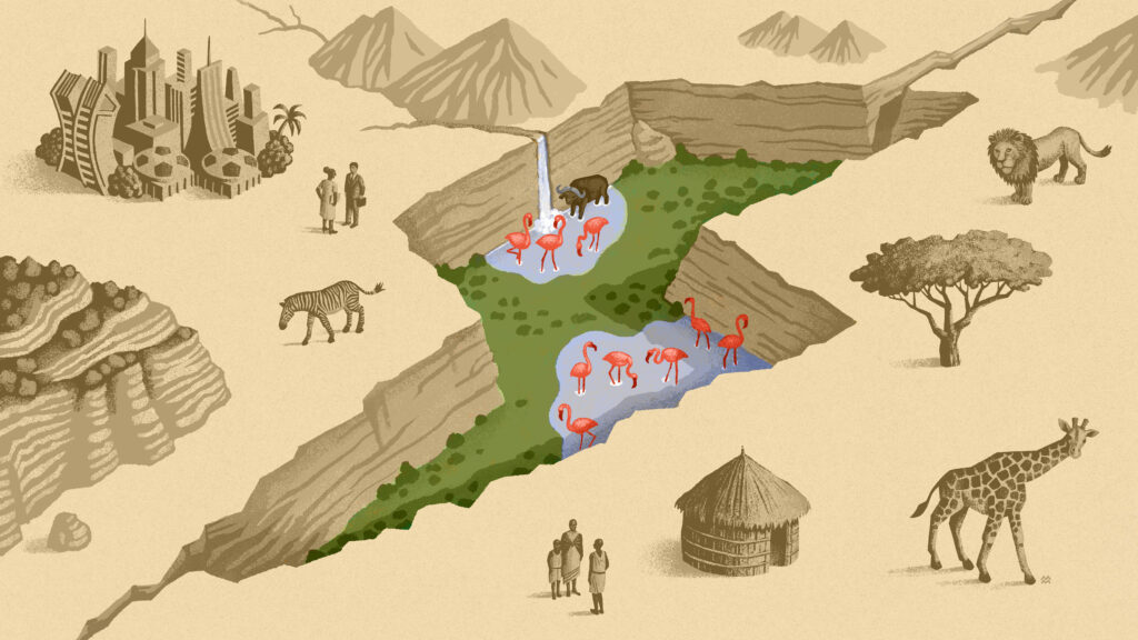
This is today’s edition of The Download, our weekday newsletter that provides a daily dose of what’s going on in the world of technology. Three reasons why DeepSeek’s new model matters On Friday, Chinese AI firm DeepSeek released a preview of V4, its long-awaited new flagship model. Notably, the model can process much longer prompts than its last generation, thanks to a new design that handles large amounts of text more efficiently. While the model remains open source, its performance matches leading closed-source rivals from Anthropic, OpenAI, and Google. It is also DeepSeek’s first release optimized Huawei’s Ascend chips—a key test of China’s dependence on Nvidia. Here are three ways V4 could shake up AI. —Caiwei Chen The rise of world models AI systems have already gained impressive mastery over the digital world, but the physical world remains humanity’s domain. As it turns out, building an AI that composes novels or code apps is far easier than developing one to fold laundry or navigate city streets. To bridge this gap, many researchers believe you need something called a world model. Proponents like Stanford professor Fei-Fei Li and AMI Labs founder Yann LeCun argue these models can overcome the well-known limitations of LLMs—and realize AI’s promise for robotics. Find out why they’ve brought world models to the forefront of the field. —Grace Huckins World models are on our list of the 10 Things That Matter in AI Right Now, our essential guide to what’s really worth your attention in the field. Subscribers can watch an exclusive roundtable unveiling the technologies and trends on the list, with analysis from MIT Technology Review’s AI reporter Grace Huckins and executive editors Amy Nordrum and Niall Firth. The must-reads I’ve combed the internet to find you today’s most fun/important/scary/fascinating stories about technology. 1 China has blocked Meta’s $2 billion acquisition of AI startup ManusRegulators cited national security grounds. (WSJ $)+ Beijing called the deal a “conspiratorial” attempt to hollow out its tech base. (FT $)+ The country is tightening its grip on AI firms that try to leave. (TechCrunch)+ The decision escalates China’s AI rivalry with the US. (Bloomberg $)+ But there will be no winners in their competition. (MIT Technology Review) 2 Google is investing up to $40 billion in AnthropicIn a deal valuing the AI firm at $350 billion. (CNBC)+ The funding will support the firm’s growing computing needs. (TechCrunch)+ Anthropic and OpenAI are fighting for compute capacity. (Axios) 3 President Trump just fired the entire National Science BoardThe NSF has played a crucial role in developing technology. (The Verge)+ The move heightens fears over political interference in US science. (Nature) 4 Conspiracy theories about the Washington shooting are proliferating onlineOver 300,000 posts appeared on X using the keyword “staged.” (NYT $)+ The theories are also swirling on Bluesky and Instagram. (Wired) 5 The AI compute crunch is starting to hit the broader economy.It’s affecting jobs, gadgets, and electricity prices. (404 Media)+ The AI compute explosion is the tech story of our time. (MIT Technology Review) 6 Elon Musk says a new banking tool brings X close to a “super app”He’s pledged to launch the tool this month. (Bloomberg) 7 AI optimism is surging across Asia while US sentiment coolsThe divide could shape where adoption happens fastest. (Rest of World) 8 Apple is tying its new CEO’s ascent to its first foldable iPhoneIt wants to build the buzz around John Ternus. (Gizmodo)  9 Twelve firms are developing the Golden Dome’s space-based interceptorsThey’ve won contracts worth up to $3.2 billion. (Ars Technica) 10 NASA has shared promising results from Artemis IIThe spacecraft and rocket fared well. (Engadget) Quote of the day “Getting out the truth and establishing facts and reliable information takes time. But our audiences really don’t have that kind of patience.” —Amanda Crawford, associate professor at the University of Connecticut, tells the NYT why conspiracy theories are gaining traction online. One More Thing MIRIAM MARTINCIC Welcome to Kenya’s Great Carbon Valley: a bold new gamble to fight climate change Kenya’s Great Rift Valley is home to five geothermal power stations, which harness clouds of steam to generate about a quarter of the country’s electricity. But some of the energy escapes into the atmosphere, while even more remains underground for lack of demand. That’s what brought Octavia Carbon here. Last year, the startup began harnessing some of that excess energy to remove CO2 from the air. The company says the method is efficient, affordable, and—crucially—scalable. But the project also faces fierce opposition.  Read the full story on the future of Kenya’s “Great Carbon Valley.” —Diana Kruzman We can still have nice things A place for comfort, fun and distraction to brighten up your day. (Got any ideas? Drop me a line.) + Fred Again’s Tiny Desk Concert is a masterclass in intimate performance.+ Here’s a delightful look at how we’re all linked through geography and shared heritage.+ Take a short, peaceful break to watch Tokyo’s cherry blossoms from a bird’s eye view.+ There’s something oddly satisfying about watching an industrial shredder turn everyday items into confetti.

In a

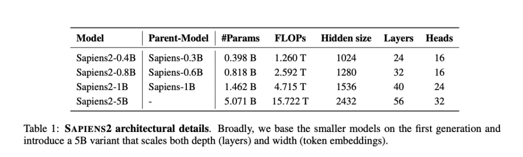
If you’ve ever watched a motion capture system struggle with a person’s fingers, or seen a segmentation model fail to distinguish teeth from gums, you already understand why human-centric computer vision is hard. Humans are not just objects, they come with articulated structure, fine surface details, and enormous variation in pose, clothing, lighting, and ethnicity. Getting a model to understand all of that, at once, across arbitrary real-world images, is genuinely difficult. Meta AI research team introduced Sapiens2, the second generation of its foundation model family for human-centric vision. Trained on a newly curated dataset of 1 billion human images, spanning model sizes from 0.4B to 5B parameters, and designed to operate at native 1K resolution with hierarchical variants supporting 4K, Sapiens2 is a substantial leap over its predecessor across every benchmark the team evaluated. https://arxiv.org/pdf/2604.21681 What Sapiens2 is Trying to Solve The original Sapiens model relied primarily on Masked Autoencoder (MAE) pretraining. MAE works by masking a large portion of input image patches, 75% in this case, and training the model to reconstruct the missing pixels. This forces the model to learn spatial details and textures, which is useful for dense prediction tasks like segmentation or depth estimation. The problem is that MAE, as a form of masked image modeling (MIM), learns largely through compression. It doesn’t naturally learn high-level semantics. It can tell you what something looks like, but not necessarily what it means in the context of a human body. That’s where contrastive learning (CL) methods like DINO and SimCLR shine: they organize representations semantically by training the model to treat different views of the same image as similar and views of different images as distinct. But CL has its own tradeoff. Its aggressive augmentation strategies like color jitter, blurring, can strip away appearance cues like skin tone or lighting conditions that are critical for tasks like albedo estimation (recovering the true color of a surface independent of lighting). This is what the research team calls representation drift. Sapiens2 addresses this problem directly by combining both objectives: a masked image reconstruction loss (LMAE) to preserve low-level fidelity, and a global contrastive loss (LCL) on the [CLS] token using a student-teacher framework based on DINOv3, where the teacher’s parameters are an exponential moving average (EMA) of the student. Crucially, color augmentations are not applied to global views used for the MAE objective, preserving the appearance cues needed for photorealistic tasks. The joint objective is L = LMAE + λLCL. https://arxiv.org/pdf/2604.21681 The Data: Humans-1B Getting 1 billion training images right required a multi-stage filtering pipeline. Starting from a web-scale pool of approximately 4 billion images, Meta team applied bounding box detection, head-pose estimation, aesthetic and realism scoring, CLIP-based feature filtering, and text-overlay detection. The result is a curated corpus where every image contains at least one prominent person with a minimum short-side resolution of 384 pixels. To ensure diversity, the research team used perceptual hashing and deep-feature nearest-neighbor pruning for deduplication, then clustered visual embeddings and applied selective sampling to balance the dataset across poses, viewpoints, occlusion levels, clothing types, and lighting conditions. No task labels or human-specific priors were injected during pretraining — just images. The Architecture: Scaling to 5B and 4K Sapiens2 introduces four model sizes: 0.4B, 0.8B, 1B, and 5B parameters, each at native 1K resolution. The 5B model is the highest-FLOPs vision transformer reported to date at 15.722 TFLOPs. For 4K resolution, the research team adopted a hierarchical windowed attention design. The first K layers apply windowed self-attention locally to capture fine texture and boundaries within spatial windows. A [CLS]-guided pooling step then downsamples the 2D token grid by a spatial stride √ω, and the subsequent L layers apply global self-attention over this reduced sequence. This layout is compatible with MAE-style pretraining because masked tokens can be dropped after the local stage, preventing information from leaking across masked regions — a problem that convolutional backbones typically need masked convolutions to avoid. The masking strategy itself is also carefully designed: Sapiens2 uses mixed blockwise/patchwise masking (blockwise probability 0.4) at a 75% mask ratio with patch size 16. At 1024×768 resolution (64×48 = 3072 patches), this masks approximately 2304 patches per image which is enough to create coarse occlusions that regularize MAE while preserving sufficient context for the contrastive objective. For stability at scale, the architecture incorporates several improvements: RMSNorm replacing LayerNorm, Grouped-Query Attention (GQA) in mid-depth blocks for higher throughput, QK-Norm for robust high-resolution training, and SwiGLU feed-forward layers. The decoder uses pixel-shuffle upsampling for sub-pixel reasoning. Decoder output resolution was also increased from 0.5K to 1K for base backbones, and to 2K for 4K backbones. Post-Training: Five Human Tasks, 10× More Supervision A critical improvement over the original Sapiens is the scale and quality of task-specific supervision. Relative to the first generation, Sapiens2 scales task-specific labels by 10×, typically reaching around 1 million labels per task. After pretraining, the backbone is fine-tuned for five downstream tasks using lightweight task-specific heads while leaving the backbone unchanged: Pose Estimation: A 308-keypoint full-body skeleton with dense face (243 keypoints) and hand (40 keypoints) coverage. The research team newly annotated 100K in-the-wild images to complement studio capture data, improving generalization significantly. Body-Part Segmentation: 29 semantic classes (extended from 28 by adding eyeglasses), trained with per-pixel weighted cross-entropy combined with Dice loss for sharper boundaries. Pointmap Estimation: Rather than predicting relative depth, Sapiens2 regresses a per-pixel 3D pointmap P̂(u) ∈ ℝ³ in the camera frame — a harder task that requires reasoning about camera intrinsics. Normal Estimation: Per-pixel surface unit normals, decoded using multiple PixelShuffle layers for artifact-free upsampling. Albedo Estimation: Per-pixel diffuse albedo Â(u) ∈ [0,1]³, trained purely on synthetic high-fidelity data and designed to recover true skin tone and clothing color under varying illumination. Results The numbers are difficult to argue with. On the 11K-image in-the-wild pose test set, Sapiens2-5B achieves 82.3 mAP compared to 78.3 mAP for Sapiens-2B — a +4 mAP improvement. On body-part segmentation, even the smallest model, Sapiens2-0.4B, scores 79.5 mIoU (+21.3 over

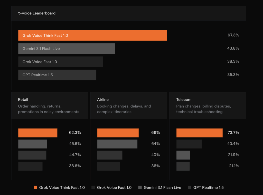
Building a production-grade voice AI agent is one of the hardest engineering challenges in applied machine learning today. It is not just about transcription accuracy. You need a system that can hold context across a five-minute conversation, invoke external APIs mid-call without an awkward pause, gracefully recover when a caller corrects themselves, and do all of this reliably when the audio is degraded by background noise, a heavy accent, or a dropped word. Most current systems handle one or two of those requirements. xAI’s newly released grok-voice-think-fast-1.0 is making a serious claim to handle all of them — and the benchmark numbers back it up. Available via the xAI API, grok-voice-think-fast-1.0 is the xAI’s new flagship voice model. It is purpose-built for complex, ambiguous, multi-step workflows across customer support, sales, and enterprise applications, and it is already deployed at scale powering Starlink’s live phone operations. What Makes a Voice Agent Full-Duplex? Before unpacking the benchmark results, it is worth understanding what kind of model grok-voice-think-fast-1.0 is. It is evaluated on the (Tau) τ-voice Bench as a full-duplex voice agent. The system processes incoming speech and generates responses simultaneously, rather than waiting for the speaker to stop before it begins thinking. This is how humans communicate in real conversations. It is also why handling interruptions is a genuinely hard technical problem: the model must decide in real time whether a mid-sentence utterance is a correction, a clarification, or just a filler word, and adjust its behavior accordingly. The τ-voice Bench evaluates agents specifically under these realistic conditions: noise, accents, interruptions, and natural turn-taking, making it a more relevant measure for production deployments than traditional clean-audio ASR benchmarks. https://x.ai/news/grok-voice-think-fast-1 The Numbers: A Significant Lead The benchmark results xAI published are striking in how large the gaps are. On the τ-voice Bench overall leaderboard, grok-voice-think-fast-1.0 scores 67.3%, compared to 43.8% for Gemini 3.1 Flash Live, 38.3% for Grok Voice Fast 1.0 (xAI’s own previous model), and 35.3% for GPT Realtime 1.5. Breaking that down by vertical tells an even clearer story: In Retail — covering order handling, returns, and promotions in noisy environments — grok-voice-think-fast-1.0 scores 62.3%, followed by Grok Voice Fast 1.0 at 45.6%, Gemini 3.1 Flash Live at 44.7%, and GPT Realtime 1.5 at 38.6%. In Airline — booking changes, delays, and complex itineraries — the scores are 66% for Grok Voice Think Fast 1.0, 64% for Grok Voice Fast 1.0, 40% for Gemini 3.1 Flash Live, and 36% for GPT Realtime 1.5. The most dramatic gap appears in Telecom: plan changes, billing disputes, and technical troubleshooting — where grok-voice-think-fast-1.0 achieves 73.7%, while Grok Voice Fast 1.0 scores 40.4%, Gemini 3.1 Flash Live 21.9%, and GPT Realtime 1.5 21.1%. A 33-percentage-point lead over the next competitor in a single vertical is not a marginal improvement. That is an architectural advantage. Real-Time Reasoning With Zero Added Latency One of the most technically significant design decisions in this model is how reasoning is handled. grok-voice-think-fast-1.0 performs reasoning in the background, thinking through challenging queries and workflows in real time with no impact on response latency. For AI teams, this is the difficult part to build: reasoning models traditionally increase response time because they generate intermediate ‘thinking’ tokens before producing an answer. Hiding that computation from the conversational latency budget, while still benefiting from it, requires careful architecture work. The practical payoff is accuracy without sluggishness. xAI team demonstrates this with a representative edge case: when asked “Which months of the year are spelled with the letter X?”, grok-voice-think-fast-1.0 correctly responds that no month contains the letter X. On the other hand, the competing models confidently and incorrectly answered “February.” This class of error, where a model produces a plausible-sounding but wrong answer with high confidence, is particularly damaging in voice interfaces because users have no text output to cross-check. Precise Data Entry and Read-Back A core workflow capability of grok-voice-think-fast-1.0 is structured data capture and read-back. The model can seamlessly collect email addresses, physical street addresses, phone numbers, full names, account numbers, and other structured data, even when information is spoken quickly or with a strong accent. It gracefully handles speech disfluencies and accepts natural corrections as a human would, then reads back the confirmed data to the user. xAI illustrates this with a concrete example. A caller says: “Yep, it’s 1410, uh wait, 1450 Page Mill Street. Actually no sorry, that’s Page Mill Road.” The model processes the spoken corrections in real time, invokes a search_address tool with the corrected parameter “1450 Page Mill Rd”, and reads back the normalized address for user confirmation. Data teams who has spent time building post-call cleanup pipelines to extract structured fields from messy transcripts, this native capture-and-read-back capability represents a meaningful reduction in downstream processing complexity. The model has been battle-tested in the toughest real-world conditions: telephony audio, background noise, heavy accents, and frequent interruptions. It natively supports 25+ languages, making it ideal for global deployments across use cases including customer support, phone sales, appointment booking, and restaurant reservations. The Starlink Deployment: Production at Scale The most compelling validation of grok-voice-think-fast-1.0 is not the benchmark alone but it’s live deployment. Grok Voice powers the full phone sales and customer support operation for Starlink at +1 (888) GO STARLINK. The numbers xAI discloses from this deployment are operationally significant: a 20% sales conversion rate (meaning one in five callers making a sales inquiry purchases Starlink service while on the phone with Grok), a 70% autonomous resolution rate for customer support inquiries with no human in the loop, and a single agent operating across 28 distinct tools spanning hundreds of support and sales workflows. Key Takeaways grok-voice-think-fast-1.0 leads the τ-voice Bench with a 67.3% score, outperforming Gemini 3.1 Flash Live (43.8%), Grok Voice Fast 1.0 (38.3%), and GPT Realtime 1.5 (35.3%). The model performs background reasoning with zero added latency, allowing it to think through complex, multi-step workflows in real time without slowing down conversational responses. Precise data entry and read-back is a native capability, enabling

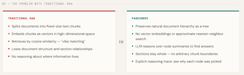
Retrieval is where most RAG systems quietly break. Traditional pipelines rely on vector similarity—embedding queries and document chunks into the same space and fetching the “closest” matches. But similarity is a weak proxy for what we actually need: relevance grounded in reasoning. In long, professional documents—like financial reports, research papers, or legal texts—the right answer often isn’t in the most semantically similar paragraph. It requires navigating structure, understanding context, and performing multi-step reasoning across sections. This is exactly where vector-based RAG starts to fall apart. PageIndex is designed to solve this gap by rethinking retrieval from first principles. Instead of chunking documents and searching via embeddings, it builds a hierarchical table-of-contents-style tree index and uses LLMs to reason over that structure—much like a human expert scanning sections, drilling down, and connecting ideas. This enables a vectorless, reasoning-driven retrieval process that is more interpretable, traceable, and aligned with how knowledge is actually extracted from complex documents. By replacing similarity search with structured exploration and tree-based reasoning, PageIndex delivers significantly higher retrieval accuracy—demonstrated by its strong performance on benchmarks like FinanceBench—making it particularly effective for domains that demand precision and deep understanding. In this article, we’ll use PageIndex to index the seminal Transformer paper — “Attention Is All You Need” — and run two cross-cutting queries against it without a single vector or embedding. Instead of chunking the PDF and retrieving by similarity, PageIndex builds a hierarchical tree of the document’s sections, then uses GPT-5.4 to reason over node summaries and identify exactly which sections contain the answer — before reading a single word of full text. Setting up the dependencies For this tutorial, you would require PageIndex & OpenAI API keys. You can get the same from https://dash.pageindex.ai/api-keys and https://platform.openai.com/api-keys respectively. Copy CodeCopiedUse a different Browser pip install pageindex openai requests Copy CodeCopiedUse a different Browser from pageindex import PageIndexClient import pageindex.utils as utils import os from getpass import getpass PAGEINDEX_API_KEY = getpass(‘Enter PageIndex API Key: ‘) pi_client = PageIndexClient(api_key=PAGEINDEX_API_KEY) We import the OpenAI client and configure it with an API key to enable access to LLMs. Then, we define an asynchronous helper function that sends prompts to the model and returns the generated response. Copy CodeCopiedUse a different Browser import openai OPENAI_API_KEY = getpass(‘Enter OpenAI API Key: ‘) async def call_llm(prompt, model=”gpt-5.4″, temperature=0): client = openai.AsyncOpenAI(api_key=OPENAI_API_KEY) response = await client.chat.completions.create( model=model, messages=[{“role”: “user”, “content”: prompt}], temperature=temperature ) return response.choices[0].message.content.strip() Building the PageIndex Tree In this chunk, we download the Transformer paper directly from arXiv and submit it to PageIndex, which processes the PDF and builds a hierarchical tree of its sections — each node storing a title, a summary, and the full section text. Once the tree is ready, we print it out to inspect the structure PageIndex has inferred: every chapter, subsection, and nested heading becomes a node in the tree, preserving the document’s natural organization exactly as the authors intended it. Copy CodeCopiedUse a different Browser # ───────────────────────────────────────────── # Step 1: Build the PageIndex Tree # ───────────────────────────────────────────── # 1.1 Download the Transformer paper and submit it import os, requests pdf_url = “https://arxiv.org/pdf/1706.03762.pdf” pdf_path = os.path.join(“data”, pdf_url.split(“/”)[-1]) os.makedirs(“data”, exist_ok=True) print(“Downloading ‘Attention Is All You Need’…”) response = requests.get(pdf_url) with open(pdf_path, “wb”) as f: f.write(response.content) print(f” Saved to {pdf_path}”) doc_id = pi_client.submit_document(pdf_path)[“doc_id”] print(f” Document submitted. doc_id: {doc_id}”) # 1.2 Retrieve the tree (poll until ready) import time print(“nWaiting for PageIndex tree to be ready”, end=””) while not pi_client.is_retrieval_ready(doc_id): print(“.”, end=””, flush=True) time.sleep(5) tree = pi_client.get_tree(doc_id, node_summary=True)[“result”] print(“nn Document Tree Structure:”) utils.print_tree(tree) Reasoning-Based Retrieval With the tree built, we now run a query that is intentionally cross-cutting — one that can’t be answered by a single section of the paper. We strip the full text from each node, leaving only titles and summaries, and pass the entire tree structure to GPT-5.4. The model then reasons over these summaries to identify every node likely to contain a relevant answer, returning both its step-by-step thinking and a list of matched node IDs. This is the core of what makes PageIndex different: the LLM decides where to look before any full text is loaded. Copy CodeCopiedUse a different Browser # ───────────────────────────────────────────── # Step 2: Reasoning-Based Retrieval # ───────────────────────────────────────────── # 2.1 Define a query that requires navigating across sections import json # This query is intentionally cross-cutting — it can’t be answered # by a single section, which is where tree search shines over top-k. query = “Why did the authors choose self-attention over recurrence, and what are the complexity trade-offs they compared?” tree_without_text = utils.remove_fields(tree.copy(), fields=[“text”]) search_prompt = f””” You are given a question and a hierarchical tree structure of a research paper. Each node has a node_id, title, and a summary of its content. Your task: identify ALL nodes that are likely to contain information relevant to answering the question. Think carefully — the answer may be spread across multiple sections. Question: {query} Document tree: {json.dumps(tree_without_text, indent=2)} Reply ONLY in this JSON format, no preamble: {{ “thinking”: “<step-by-step reasoning about which nodes are relevant and why>”, “node_list”: [“node_id_1”, “node_id_2”, …] }} “”” print(f’ Query: “{query}”n’) print(“Running tree search with GPT-5.4…”) tree_search_result = await call_llm(search_prompt) # 2.2 Inspect the retrieval reasoning and matched nodes node_map = utils.create_node_mapping(tree) result_json = json.loads(tree_search_result) print(“n LLM Reasoning:”) utils.print_wrapped(result_json[“thinking”]) print(“n Retrieved Nodes:”) for node_id in result_json[“node_list”]: node = node_map[node_id] print(f” • [{node[‘node_id’]}] Page {node[‘page_index’]:>2} — {node[‘title’]}”) Answer Generation Once the relevant nodes are identified, we pull their full text and stitch it together into a single context block — each section clearly labeled so the model knows where each piece of information comes from. That combined context is then handed to GPT-5.4 with a structured prompt that asks for the core motivation, the specific complexity numbers, and any caveats the authors acknowledged. The model answers using only what was retrieved, grounding every claim directly in the paper’s text. Copy CodeCopiedUse a different Browser # ───────────────────────────────────────────── # Step 3: Answer Generation # ───────────────────────────────────────────── # 3.1 Stitch together context from all retrieved nodes node_list = result_json[“node_list”] relevant_content = “nn—nn”.join( f”[Section: