YouZum

Uncategorized

AI, Committee, ข่าว, Uncategorized

China’s AI models have Trump’s AI world at war with itself

This story originally appeared in The Algorithm, our weekly newsletter on AI. To get stories like this in your inbox first, sign up here. Over the weekend, several current and former advisors to President Donald Trump on AI publicly lobbed insults at the country’s leading AI companies. David Sacks, the president’s AI and crypto “czar” until March, branded Anthropic’s models as “lobotomized” and “woke.” Emil Michael, a top Pentagon official, called OpenAI’s new head of strategic futures a “supreme village idiot.” It began because no one can agree on what to do about Kimi, a free, open source model that Chinese AI company Moonshot launched last week. It appears to rival the intelligence of models from OpenAI and Anthropic, which are very much not free.  Kimi and other Chinese models like it pose a real problem for Trump. And they’re dividing the top AI strategists in his orbit into factions. Every time a new smart, free model from China like Kimi gets released, US companies see less reason to fork out money to access models from Anthropic or OpenAI. Given that enthusiasm for these and other AI companies is driving an outsized share of economic growth, China’s AI models create both economic and political problems for the president. They are “a threat for an administration that really doesn’t want more economic bad news,” Anton Leicht, a fellow at the Carnegie Endowment, wrote on X. They’ve already rattled US stocks.  What is Trump to do? First, consider that this is all happening just a week after New York imposed the country’s first state ban on new data centers. There is growing distrust of AI companies, and I imagine a not-insignificant share of Americans would have little sympathy for OpenAI or Anthropic as they fend off cheaper competitors, and would say it’s not the government’s job to protect their interests. On this point, they’d see a sliver of agreement (and really just a sliver) with David Sacks, who on July 19 criticized top AI companies that “want the government to eliminate their open source competition.” He has also argued that Chinese AI models have become popular because they come with fewer restrictions on how people can use them (putting aside the built-in state censorship).  Sacks, however, is out of a job. He no longer has a formal role advising Trump, and his position that more open AI is better has been largely replaced in the administration by one that sees a larger role for government intervention. The thinking behind this view is that because AI models have gotten strong enough to pose threats to national security, the government must control how they’re used.  This position has fueled the new White House review process that aims to vet AI models’ security before they’re released. Dean Ball, a former Trump AI advisor who now works for OpenAI, criticized it over the weekend as a “de facto licensing regime for frontier AI.” Ball predicted Trump may solve his Chinese open source problem with a bit of soft power, perhaps by making US companies afraid to use models like Kimi. That drew a response from Michael, who, with Secretary of Defense Pete Hegseth, has been the agency’s main liaison with AI companies. Michael called Ball the AI industry’s “supreme village idiot,” bristling at the suggestion that the government would quietly strong-arm companies rather than, as Michael put it, go through “the democratic process not some Deep State scheme.” Left out of the conversation has been how a model like Kimi got so good in the first place. For much of the Biden administration and even the beginning of Trump’s second administration, keeping China from getting top chips was a priority. Those export controls have loosened—Trump made the controversial decision to allow Nvidia to sell more chips to China, in exchange for the US government taking a cut—and the government has alleged that some chip smuggling has taken place. But China nonetheless has limited computing power, and it’s not clear what chips the company behind Kimi used to train the model.  It’s possible that the process involved some distillation, a practice in which AI models are trained on the outputs of existing AI models. OpenAI and Anthropic have long complained that Chinese AI companies do this, and they have requested government help to put a stop to it. In April, they got it, when the Trump administration announced a series of efforts to curb the practice.   But Kimi is out there and free, and it is nearly as good as the Anthropic model the US government deemed so powerful that it was briefly shut down because it threatened national security. The weekend’s sparring suggests many in Trump’s orbit see that as a wake-up call. But nobody can agree on what for.

China’s AI models have Trump’s AI world at war with itself Read Post »
AI, Committee, ข่าว, Uncategorized

Fine-Tuning Qwen3 with LoRA Using NVIDIA NeMo AutoModel: A Complete Single-GPU Google Colab Workflow Tutorial

In this tutorial, we build an end-to-end NVIDIA NeMo AutoModel workflow in Google Colab and use a single GPU to explore the same configuration-driven training architecture that scales to distributed multi-GPU environments. We verify the available CUDA hardware and precision support, install NeMo AutoModel directly from its source repository, load an official Qwen3-0.6B LoRA fine-tuning recipe, and programmatically adapt its precision, batch-size, checkpointing, and scheduler settings for a constrained Colab runtime. We then launch parameter-efficient fine-tuning through the automodel command-line interface, locate and reload the generated LoRA checkpoint, and compare outputs from the original and fine-tuned models. Finally, we use NeMoAutoModelForCausalLM through the Python API to demonstrate how NeMo AutoModel integrates NVIDIA-optimized execution paths while preserving the familiar Hugging Face model interface. Setting Up the Colab Workspace and Shell Helper Copy CodeCopiedUse a different Browser import os, sys, glob, json, subprocess, shutil, textwrap REPO_DIR = “/content/Automodel” WORK_DIR = “/content/automodel_demo” CKPT_DIR = os.path.join(WORK_DIR, “checkpoints”) os.makedirs(WORK_DIR, exist_ok=True) def sh(cmd, check=True): print(f”n$ {cmd}n” + “-” * 78) p = subprocess.Popen(cmd, shell=True, stdout=subprocess.PIPE, stderr=subprocess.STDOUT, text=True, bufsize=1) for line in p.stdout: print(line, end=””) p.wait() if check and p.returncode != 0: raise RuntimeError(f”Command failed ({p.returncode}): {cmd}”) return p.returncode We import the core Python libraries required for file handling, process execution, path management, and formatted output. We define the repository, working, and checkpoint directories used throughout the workflow. We also create a reusable shell-command function that streams command output and raises errors when execution fails. Verifying the GPU and Installing NeMo AutoModel Copy CodeCopiedUse a different Browser print(“=” * 78) print(“STEP 0 — Checking GPU runtime”) print(“=” * 78) import torch assert torch.cuda.is_available(), ( “No GPU found! In Colab: Runtime -> Change runtime type -> select a GPU.” ) GPU_NAME = torch.cuda.get_device_name(0) BF16_OK = torch.cuda.is_bf16_supported() VRAM_GB = torch.cuda.get_device_properties(0).total_memory / 1e9 print(f”GPU: {GPU_NAME} | VRAM: {VRAM_GB:.1f} GB | bf16 supported: {BF16_OK}”) print(“n” + “=” * 78) print(“STEP 1 — Installing NeMo AutoModel (takes a few minutes)”) print(“=” * 78) if not os.path.isdir(REPO_DIR): sh(f”git clone –depth 1 https://github.com/NVIDIA-NeMo/Automodel.git {REPO_DIR}”) sh(f”pip -q install -e {REPO_DIR}”) sh(“pip -q install pyyaml peft”) sh(‘python -c “import nemo_automodel; print(‘NeMo AutoModel version:’, ‘ ‘getattr(nemo_automodel, ‘__version__’, ‘source’))”‘) We verify that the Colab runtime provides a CUDA-enabled GPU and inspect its name, memory capacity, and bfloat16 support. We clone the NVIDIA NeMo AutoModel repository when it is not already available and install the package directly from source. We then install the supporting YAML and PEFT libraries and confirm that the NeMo AutoModel package imports correctly. Loading and Patching the Qwen3 LoRA Recipe Copy CodeCopiedUse a different Browser print(“n” + “=” * 78) print(“STEP 2 — Preparing the recipe”) print(“=” * 78) import yaml candidates = sorted(glob.glob( os.path.join(REPO_DIR, “examples”, “llm_finetune”, “qwen”, “*0p6b*peft*.yaml”) )) or sorted(glob.glob( os.path.join(REPO_DIR, “examples”, “llm_finetune”, “**”, “*peft*.yaml”), recursive=True, )) assert candidates, “Could not find a PEFT recipe in the cloned repo.” BASE_RECIPE = candidates[0] print(f”Base recipe: {os.path.relpath(BASE_RECIPE, REPO_DIR)}”) with open(BASE_RECIPE) as f: cfg = yaml.safe_load(f) print(“n— Original recipe (as shipped) —“) print(yaml.dump(cfg, sort_keys=False)[:2500]) def patch(node): if isinstance(node, dict): for k, v in list(node.items()): if isinstance(v, str) and not BF16_OK and v.lower() in ( “bf16”, “bfloat16”, “torch.bfloat16”): node[k] = “float32” elif k in (“batch_size”, “local_batch_size”) and isinstance(v, int): node[k] = min(v, 4) elif k == “global_batch_size” and isinstance(v, int): node[k] = min(v, 8) else: patch(v) elif isinstance(node, list): for item in node: patch(item) patch(cfg) cfg.setdefault(“step_scheduler”, {}) cfg[“step_scheduler”][“max_steps”] = 40 cfg[“step_scheduler”][“ckpt_every_steps”] = 40 cfg[“step_scheduler”][“num_epochs”] = 1 if isinstance(cfg.get(“checkpoint”), dict): cfg[“checkpoint”][“enabled”] = True cfg[“checkpoint”][“checkpoint_dir”] = CKPT_DIR DEMO_RECIPE = os.path.join(WORK_DIR, “qwen3_0p6b_colab_lora.yaml”) with open(DEMO_RECIPE, “w”) as f: yaml.dump(cfg, f, sort_keys=False) print(“n— Patched recipe (what we will actually run) —“) print(yaml.dump(cfg, sort_keys=False)[:2500]) MODEL_ID = “Qwen/Qwen3-0.6B” try: MODEL_ID = cfg[“model”][“pretrained_model_name_or_path”] except Exception: pass print(f”nBase model: {MODEL_ID}”) We locate an official PEFT recipe, load its YAML configuration, and inspect the original training settings. We recursively adapt the precision and batch size parameters to fit the recipe on a single Colab GPU while preserving its original structure. We also limit the training duration, configure checkpoint output, save the patched recipe, and extract the Hugging Face model identifier. Running LoRA Fine-Tuning on HellaSwag Copy CodeCopiedUse a different Browser print(“n” + “=” * 78) print(“STEP 3 — Training (LoRA fine-tune of Qwen3-0.6B on HellaSwag)”) print(“=” * 78) env_prefix = “HF_HUB_ENABLE_HF_TRANSFER=0 TOKENIZERS_PARALLELISM=false” rc = sh(f”cd {WORK_DIR} && {env_prefix} automodel {DEMO_RECIPE}”, check=False) if rc != 0: print(“nRetrying with legacy CLI syntax…”) sh(f”cd {WORK_DIR} && {env_prefix} automodel finetune llm -c {DEMO_RECIPE}”) We launch Qwen3-0.6B LoRA fine-tuning on the HellaSwag dataset through the NeMo AutoModel command-line interface. We turn off unnecessary Hugging Face transfer and tokenizer parallelism features to keep the Colab run more predictable. We also include a fallback command that supports older NeMo AutoModel CLI syntax when the primary invocation fails. Comparing Base and Fine-Tuned Model Outputs Copy CodeCopiedUse a different Browser print(“n” + “=” * 78) print(“STEP 4 — Evaluating: base model vs LoRA fine-tuned model”) print(“=” * 78) from transformers import AutoModelForCausalLM, AutoTokenizer DTYPE = torch.bfloat16 if BF16_OK else torch.float32 PROMPT = (“A man is sitting on a roof. He starts pulling up roofing shingles. ” “What happens next?”) def generate(model, tok, prompt, max_new_tokens=60): inputs = tok(prompt, return_tensors=”pt”).to(model.device) with torch.no_grad(): out = model.generate(**inputs, max_new_tokens=max_new_tokens, do_sample=False, temperature=None, top_p=None, pad_token_id=tok.eos_token_id) return tok.decode(out[0][inputs[“input_ids”].shape[1]:], skip_special_tokens=True) tok = AutoTokenizer.from_pretrained(MODEL_ID) base = AutoModelForCausalLM.from_pretrained( MODEL_ID, torch_dtype=DTYPE, device_map=”cuda”) print(“n[BASE MODEL]”) print(textwrap.fill(generate(base, tok, PROMPT), 90)) ckpt_glob = sorted(glob.glob(os.path.join(CKPT_DIR, “**”, “model”), recursive=True)) if not ckpt_glob: ckpt_glob = sorted(glob.glob(os.path.join(WORK_DIR, “**”, “adapter_model.safetensors”), recursive=True)) ckpt_glob = [os.path.dirname(p) for p in ckpt_glob] if ckpt_glob: ADAPTER_DIR = ckpt_glob[-1] print(f”nFound checkpoint: {ADAPTER_DIR}”) try: from peft import PeftModel tuned = PeftModel.from_pretrained(base, ADAPTER_DIR) print(“n[FINE-TUNED MODEL (base + LoRA adapter)]”) print(textwrap.fill(generate(tuned, tok, PROMPT), 90)) except Exception as e: print(f”nCould not auto-load the adapter with peft ({e}).”) print(“Inspect the checkpoint contents manually:”) for p in glob.glob(os.path.join(ADAPTER_DIR, “*”))[:20]: print(” “, p) else: print(“nNo checkpoint found — check the training logs above.”) del base torch.cuda.empty_cache() We load the tokenizer and base causal language model, generate a deterministic response, and establish a baseline for comparison. We search the training output directories for the latest LoRA checkpoint or adapter files created during fine-tuning. We then attach the adapter with

Fine-Tuning Qwen3 with LoRA Using NVIDIA NeMo AutoModel: A Complete Single-GPU Google Colab Workflow Tutorial Read Post »

AI, Committee, ข่าว, Uncategorized

Kimi K3 vs DeepSeek V4 Pro vs GLM-5.2: Open Trillion-Scale MoE Models Compared on Benchmarks, License, and Serving Cost

Three Chinese labs now hold the top of the open-weight leaderboard. Moonshot AI’s Kimi K3, DeepSeek V4 Pro, and Zhipu AI’s GLM-5.2 are all sparse Mixture-of-Experts (MoE) models with million-token context windows. Each targets long-horizon coding and agent workloads. This article compares them on three axes an AI team actually decides on: measured capability, license terms, and serving cost. ‘Trillion-parameter’ fits Kimi K3 (2.8T) and DeepSeek V4 Pro (1.6T). GLM-5.2 is 744B total, so it is the smallest of the three by total parameters. It earns its place because it led the open-weight field before K3 shipped. The three contenders Kimi K3 is a 2.8-trillion-parameter Stable LatentMoE model activating 16 of 896 experts per token. Moonshot has not published the exact active-parameter count. K3 adds native vision, a 1M-token context window, and always-on reasoning. Moonshot calls it the first open 3T-class model. Our launch coverage is here. DeepSeek V4 Pro is a 1.6-trillion-parameter MoE with 49B active parameters, using 384 routed experts plus one shared expert. It carries a 1M-token context window with 384K max output. A smaller V4 Flash variant (284B total, 13B active) covers cheaper workloads. Weights are on Hugging Face. GLM-5.2 is a 744-billion-parameter MoE with roughly 40B active parameters and a 1M-token context window. Zhipu ships it with High and Max reasoning modes. It comes with API access Spec Kimi K3 DeepSeek V4 Pro GLM-5.2 Total parameters 2.8T 1.6T 744B (753B per Artificial Analysis) Active parameters Not disclosed (16/896 experts) 49B ~40B Context window 1M 1M (384K max output) 1M (131K max output) Modality Text + vision + video Text Text Released July 16, 2026 April 24, 2026 June 13, 2026 Benchmarks Vendor-reported scores use different harnesses, so per-benchmark numbers rarely line up cleanly across labs. The neutral comparator is the Artificial Analysis Intelligence Index, which scores all three on the same suite. On that index, Kimi K3 scores about 57, DeepSeek V4 Pro (Max reasoning) scores 44, and GLM-5.2 scores 51. K3 ranks #3 overall, behind only Claude Fable 5 and GPT-5.6 Sol, and comparable to Opus 4.8 and GPT-5.5. GLM-5.2 held the top open-weight spot until K3 shipped. Coding benchmarks tell a similar story with caveats. Moonshot’s own table runs K3 and GLM-5.2 through matched harnesses. There, K3 leads GLM-5.2 on every shared benchmark by wide margins. Benchmark (Moonshot harness) Kimi K3 GLM-5.2 DeepSWE 67.5 46.2 Program Bench 77.8 63.7 Terminal Bench 2.1 88.3 82.7 FrontierSWE 81.2 67.3 SWE Marathon 42.0 13.0 Automation Bench 30.8 12.9 GPQA-Diamond 93.5 91.2 DeepSeek does not appear in Moonshot’s table, so its numbers come from separate testing. DeepSeek-V4-Pro-Max scores 80.6% on SWE-bench Verified, the highest open-weight result at its release and tied with Gemini 3.1 Pro. It also posts 83.5 on MRCR 1M, confirming serious long-context ability. GLM-5.2 scored 62.1 on SWE-bench Pro, edging GPT-5.5 at 58.6. So, K3 is the strongest of the three on measured capability. DeepSeek V4 Pro is competitive on isolated coding tasks. GLM-5.2 trails K3 but remains a capable open-weight option. License All three ship as open-weight models, but the practical status differs today. DeepSeek V4 Pro is MIT-licensed, with weights on Hugging Face from day one. GLM-5.2 is also MIT-licensed, with full weights on Hugging Face under the zai-org organization. Both allow unrestricted commercial use, fine-tuning, and self-hosting now. Kimi K3 is the exception. Moonshot has committed to publishing weights by July 27, 2026, expected under a Modified MIT license. Until then, K3 is usable only through the API and Kimi apps. Moonshot’s recent Modified MIT terms add one attribution clause. It triggers only above 100M monthly active users. Serving cost API list pricing separates these models sharply. Model Input ($/MTok) Output ($/MTok) Cached input Kimi K3 3.00 15.00 0.30 DeepSeek V4 Pro 0.435 0.87 ~0.0036 GLM-5.2 1.40 4.40 0.26 DeepSeek V4 Pro is the cost leader by a wide margin. At list output rates, one dollar buys roughly 1.15M output tokens from V4 Pro, about 227K from GLM-5.2, and about 67K from K3. Artificial Analysis prices every model on one blended 7:2:1 cache/input/output basis, which removes vendor framing. On that basis it lists K3 at $2.31 per 1M tokens, GLM-5.2 at $0.90, and DeepSeek V4 Pro at $0.18. On cost per task, the same source reports K3 at $0.94, GLM-5.2 at $0.32, and DeepSeek V4 Pro at $0.04. Speed also differs. Artificial Analysis measures GLM-5.2 at about 168 tokens/sec, well ahead of DeepSeek V4 Pro and Kimi K3 at about 62 each. Moonshot reports above 90% cache hits in coding workloads, which drops K3’s effective input cost to $0.30 per million. Self-hosting is a different constraint. GLM-5.2 at 744B needs over 1TB of VRAM in BF16, or roughly 8x H200 at FP8. DeepSeek V4 Pro at 1.6T needs more still. Kimi K3 is heaviest: Moonshot recommends 64 or more accelerators, putting local serving out of reach for most teams. K3 uses MXFP4 weights with MXFP8 activations for broader hardware support. Which model for which job For lowest cost per token at strong coding quality, DeepSeek V4 Pro is the clear pick. Its weights are downloadable, its license is clean, and its output price undercuts both rivals. For the highest measured capability, Kimi K3 leads, but at 5x to 17x the output price and no downloadable weights until July 27. GLM-5.2 sits between them: cheaper than K3, faster than both rivals, self-hostable today, and more capable than its size suggests. If you are planning to choose based on verification depth and license clarity favor DeepSeek and GLM now. Buyers chasing peak benchmark scores wait for K3 weights or pay the API premium. Key Takeaways Kimi K3 leads the Artificial Analysis Intelligence Index (~57, #3 overall) but stays API-only until July 27. DeepSeek V4 Pro is the cost leader: ~$0.04 per task and ~1.15M output tokens per dollar at list rates. GLM-5.2 (744B) is the smallest yet fastest (~168 t/s) and self-hostable today under MIT. All three ship 1M-token context; only DeepSeek and GLM have open weights available now. The post Kimi

Kimi K3 vs DeepSeek V4 Pro vs GLM-5.2: Open Trillion-Scale MoE Models Compared on Benchmarks, License, and Serving Cost Read Post »

AI, Committee, ข่าว, Uncategorized

10 Open-Source No-Code AI Platforms for Building LLM Apps, RAG Systems, and AI Agents

Introduction Building an LLM application no longer requires wiring orchestration code by hand. A class of open-source platforms now exposes retrieval, agents, and workflows through visual canvases, web UIs, and plain-English prompts. These tools let developers prototype in minutes and self-host for data control. This article reviews ten open-source projects across three jobs: building LLM apps, building RAG systems, and building AI agents. Each entry covers what the tool does, its core capabilities, who it suits, and its verified license and repository. HKUDS AutoAgent Repository: github.com/HKUDS/AutoAgent · License: MIT · Paper: arXiv:2502.05957 AutoAgent is a zero-code agent framework from the University of Hong Kong Data Intelligence Lab. You describe a goal in natural language. The system then constructs tools, agents, and multi-agent workflows without manual coding. It ships an agent editor, a workflow editor, and a ready-to-use research assistant mode. The project is research-backed. Its paper argues that agent frameworks exclude non-programmers, and it reports strong open-source results on the GAIA benchmark. AutoAgent also functions as an open alternative to hosted Deep Research products. It works with most major LLMs, including DeepSeek, Grok, and Gemini, and runs through a Docker-based CLI. Best for: researchers and practitioners who want to spin up agents and Deep Research-style assistants from natural language, with a paper and benchmarks behind the framework. Mintplex Labs AnythingLLM Repository: github.com/Mintplex-Labs/anything-llm · License: MIT · Site: anythingllm.com AnythingLLM is an all-in-one, self-hosted platform for RAG, agents, and document chat. It runs as a desktop app or Docker container. The design targets non-technical users while keeping a privacy-first, local-first posture. A no-code Agent Flows builder handles agent logic without scripting. Capabilities include full MCP compatibility, multi-modal input, and embeddable chat widgets. It supports 30-plus LLM providers and multiple vector databases. Documents stay in your environment, which suits teams with strict data rules. The Y Combinator-backed project uses a permissive MIT license, so commercial and multi-tenant use is straightforward. Best for: individuals and small teams that want private document Q&A, agents, and a simple deployment without stitching components together. LangChain Open Agent Platform (OAP) Repository: github.com/langchain-ai/open-agent-platform · License: MIT Open Agent Platform is LangChain’s no-code, web-based interface for building and managing LangGraph agents. It targets non-developers but stays extensible for engineers. Each agent is a configuration layered on a LangGraph graph, so power users can drop into code when needed. Core features include first-class RAG through LangConnect, tool access via MCP servers, and multi-agent orchestration through an Agent Supervisor. Authentication and access control are built in, with Supabase as the default provider. The platform ships pre-built agents, including a Tools Agent and a Supervisor, and can be forked and customized. It is a newer, smaller project than the other entries here. Best for: teams already invested in the LangChain and LangGraph ecosystem that want a GUI layer over their agents. Sim (Sim Studio) Repository: github.com/simstudioai/sim · License: Apache-2.0 · Site: sim.ai Sim is a visual, agent-first workflow builder with a Figma-like canvas. You drag blocks such as Start, Agent, Function, API, Router, and Loop to compose pipelines. An AI Copilot helps assemble workflows, and you can also build in plain English. Built-in tracing and live execution make debugging explicit. The project is Apache-2.0 licensed and YC-backed. It connects to 1,000-plus tools and every major LLM provider, and supports MCP for custom integrations. You can run the hosted version or self-host with Docker. Recent work extends it toward a broader “AI workspace” with conversational orchestration. Best for: teams that want a clean visual canvas, an AI copilot, and production traction under a permissive license. LangGenius Dify Repository: github.com/langgenius/dify · License: Modified Apache-2.0 (SaaS restricted) · Site: dify.ai · Dify is a production-oriented LLM application platform. It combines visual workflow building, RAG pipelines, agent capabilities, and LLMOps monitoring. A Prompt IDE lets you compare model outputs side by side. Fifty-plus built-in tools cover search, image generation, and computation. Dify emphasizes the full lifecycle, from prototyping to observability. Document ingestion handles formats such as PDF and PPT. The project has a large contributor base and is available as Dify Cloud or self-hosted. Note the license: it is a modified Apache-2.0 that restricts multi-tenant SaaS use and requires a commercial license for those cases. Review terms before reselling it as a service. Best for: teams building and operating production LLM apps that need prompt management, RAG, agents, and runtime monitoring in one place. FlowiseAI Flowise Repository: github.com/FlowiseAI/Flowise · License: Apache-2.0 core · Site: flowiseai.com Flowise is a drag-and-drop builder for LLM apps, built on LangChain. You assemble chatbots, RAG pipelines, and multi-agent systems on a canvas. Three builder modes, Assistant, Chatflow, and Agentflow, match rising levels of complexity. Ready-made templates shorten the path from idea to prototype. Flowise is RAG-ready and integrates with 100-plus tools, vector databases, and memory modules. Enterprise features include RBAC, audit logs, observability, and SSO/SAML. You can embed assistants via an SDK or widget. The core is Apache-2.0, but files under its enterprise directory carry a separate commercial license, so check which features you need. Deployment runs locally, in Docker, on major clouds, or through managed Flowise Cloud. Best for: developers who want the lowest barrier to a working LLM app, with an easy jump to embeddable, production-grade assistants. Langflow Repository: github.com/langflow-ai/langflow · License: MIT · Maintained by DataStax Langflow is a visual platform for building AI agents and workflows. Every flow can be exposed as an API or an MCP server, then integrated into apps on any framework. The drag-and-drop editor speeds prototyping, while full Python source access allows deep customization. Features include multi-agent orchestration and integrations with observability tools such as LangSmith and LangFuse. It supports all major LLMs, including local models, and ships a desktop app for Windows and macOS. Its permissive MIT license makes commercial and multi-tenant deployments simple. Treat it as low-code: visual by default, but code-friendly for advanced logic. Best for: developers who want a visual interface over flexible, code-extensible agent and workflow building, with strong observability options. InfiniFlow RAGFlow Repository: github.com/infiniflow/ragflow · License:

10 Open-Source No-Code AI Platforms for Building LLM Apps, RAG Systems, and AI Agents Read Post »

AI, Committee, ข่าว, Uncategorized

Zyphra Releases ZUNA1.1: An Apache 2.0 EEG Foundation Model With Variable-Length Inputs From 0.5 To 30 Seconds

This week, Zyphra released ZUNA1.1 under the Apache 2.0 license. The EEG foundation model reconstructs, denoises, and upsamples data across arbitrary channel layouts. It builds on ZUNA1, the Zyphra’s earlier open EEG foundation model. The main change is flexibility, not a jump in raw accuracy. Real EEG recordings are messy. Sessions vary in length, and channels go noisy or drop out mid-session. Montages range from four-electrode headbands to 256-channel research caps. ZUNA1 processed only fixed five-second segments. ZUNA1.1 accepts variable-length inputs from 0.5 to 30 seconds. What is ZUNA1.1? To understand that flexibility, start with what the model does. ZUNA1.1 is a 380M-parameter masked diffusion autoencoder for scalp-EEG signals. Given a subset of channels, it denoises existing EEG segments and channels. It reconstructs missing ones. It also predicts novel channel signals given physical coordinates on the scalp. The parameter count is unchanged from ZUNA1. It runs on a consumer GPU and works acceptably on CPU for many workloads. Weights sit on Hugging Face; inference and preprocessing code sit on GitHub. Install with pip install zuna. Zyphra also hosts a free browser EEG Playground, and ships all of this for research use only. How The Architecture Works That flexibility rests on tokenization. ZUNA is a transformer encoder–decoder diffusion autoencoder. It slices each channel into 0.125 second segments, which is 32 samples at 256 Hz. Each segment becomes a continuous-valued token. Tokens are serialized in channel × time order. The positional encoding is the key idea. Each token carries a 4D rotary positional encoding over (x, y, z, t). That is the electrode’s 3D scalp coordinate along with its coarse-time index. Because position, not array index, tells the model where a channel sits, ZUNA is channel-agnostic. It accepts any electrode layout, and can generate signals at positions never recorded. That capability enables arbitrary channel upsampling by location. The encoder compresses the signal into a latent. That latent conditions the decoder via adaptive-RMS norm. The decoder is trained with a rectified-flow objective. ZUNA1.1’s architectural changes targeted training stability, such as added normalization layers. What Changed From ZUNA1 Since the architecture stayed close, the differences come from training. 1. Variable-length inputs (0.5–30 seconds): ZUNA1.1 samples a segment length per training example, snapped to the 0.125 s token grid. Lengths are drawn across four bins, from very short to long. The middle 1.5–10 s range is oversampled, since it is the most common operating point. Because token counts vary, Zyphra packs multiple segments per batch up to a fixed budget. Flex attention with a sample-aware mask stops tokens attending across samples. One model therefore serves a 0.5 s snippet and a 30 s stretch without reconfiguration. 2. A richer mixture of reconstruction tasks: ZUNA1 trained on one dropout pattern: uniformly random whole channels. ZUNA1.1 trains on four. The first is whole-channel dropout, covering sparse montages and dead electrodes. The second removes short time stretches across every channel. The third removes those stretches from only some channels, clustering gaps in space and time. The fourth scatters missing values across individual points. 3. Quality-aware preprocessing and a bigger corpus: ZUNA1 made channel-quality calls at the whole-recording level, discarding usable signal. ZUNA1.1 instead computes a per-channel, per-second quality score, thresholded at load time. That grew the corpus from roughly 2M to roughly 3.5M channel-hours of public EEG data. Zyphra team also precomputes two filter variants per recording: a 0.1–45 Hz bandpass, and a 0.01 Hz highpass along with notch. Generalizing across preprocessing strategies is a stated goal, not a benchmarked result. The Results Consequently, the question is whether flexibility cost accuracy. On held-out tasks, ZUNA1.1 reaches better or essentially the same reconstruction NMSE as ZUNA1. Both clearly outperform classical spherical-spline interpolation from MNE. For fair comparison, those evaluation sets used exactly five-second samples. Zyphra also ran a region-based test. Electrodes from one brain region are deleted, then reconstructed from the remaining seven. That setup is more realistic than random channel dropping. ZUNA1.1 outperforms both spherical-spline and ZUNA1 there. Interactive Explainer To make those mechanics concrete, the demo below animates the pipeline end to end. ZUNA1 vs ZUNA1.1 Taken together, the releases differ mostly in training, not architecture. Attribute ZUNA1 ZUNA1.1 Parameters 380M 380M Architecture Transformer encoder–decoder diffusion autoencoder Same, plus extra normalization layers Input length Fixed 5 s 0.5–30 s, snapped to 0.125 s grid Token 0.125 s / 32 samples at 256 Hz Same Positional encoding 4D RoPE over (x, y, z, t) Same Decoder objective Rectified flow Rectified flow Dropout schemes in training 1 (uniform random whole-channel) 4 (channel, time, channel×time, scattered) Training corpus ~2M channel-hours ~3.5M channel-hours Quality filtering Whole-recording level Per-channel, per-second score at load time Preprocessing variants Single Two (0.1–45 Hz bandpass; 0.01 Hz highpass + notch) License Apache 2.0 Apache 2.0 Reconstruction NMSE Baseline Equal or better Running It Turning to practice, reconstruct_fif runs directly on .fif files with no .pt round-trip. The older four-step pipeline still ships alongside it. Copy CodeCopiedUse a different Browser from zuna import reconstruct_fif reconstruct_fif( input_dir=”fif_in”, output_dir=”fif_out”, figures_dir=”figures”, gpu_device=0, # GPU id, or “” for CPU segment_sec=5.0, # window length; default is 5.0, not the full 30 s montage=”standard_1020″, # fallback, used only if the file has no positions repair_channels=[“Cz”], # channel(s) to fully reconstruct target_channel_count=[“Fz”, “Pz”], # add/upsample new channels by name (or an int for auto) bad_segments=[(5, 6), (10, 11, “C3”)], # mark time spans bad (all channels, or one) sample_steps=50, # diffusion steps; note: not “diffusion_sample_steps” ) Note the defaults. segment_sec is 5.0, so the 0.5–30 s range needs setting explicitly. Electrode positions are read from the file itself. The montage argument is only a fallback when positions are absent, and channels without 3D coordinates are dropped. The reconstruction target is a union. It combines the file’s own MNE bad channels and BAD_ annotations with anything requested above. Two directories are written. full_reconstruction/ holds model output everywhere. hybrid/ keeps the original and infills only inferred cells, plus a _mask.npz. Use Cases With Examples Because masking is now flexible, several practical patterns open up.

Zyphra Releases ZUNA1.1: An Apache 2.0 EEG Foundation Model With Variable-Length Inputs From 0.5 To 30 Seconds Read Post »

AI, Committee, ข่าว, Uncategorized

Sakana AI’s Error Diffusion Trains Dale-Compliant Dual-Stream Networks, Reaching 96.7% MNIST and 61.7% CIFAR-10 Without Backpropagation

Backpropagation dominates deep learning, yet it uses a mechanism the brain likely cannot. Specifically, the backward pass needs exact transposes of forward weight matrices. This is the weight transport problem. Sakana AI’s new paper, Diffusing Blame, confronts this constraint directly. The research team trains networks that obey Dale’s principle while avoiding weight transport entirely. What is Error Diffusion? Error Diffusion (ED) is a local learning rule, first proposed by Kaneko (2000). Each weight update depends on three signals only. These are presynaptic activity, a postsynaptic activation derivative, and a single global error sign. Consequently, ED never transports transposed forward weights or uses random feedback matrices. That locality makes ED naturally compatible with Dale’s principle. However, prior work demonstrated ED only on binary classification and MNIST. The Dual-Stream Architecture To satisfy that constraint, the research team split each layer into two streams. One stream is excitatory (p), and the other is inhibitory (n). The forward pass computes excitatory-minus-inhibitory preactivations for each stream: Copy CodeCopiedUse a different Browser p_i = φ_i( +p_{i-1} Wpp − n_{i-1} Wnp + bp ) n_i = φ_i( +n_{i-1} Wnn − p_{i-1} Wpn + bn ) Here, all four weight matrices stay non-negative element-wise. The biases bp and bn are the exception, since they need not be non-negative. Moreover, the negation signs before Wnp and Wpn are structural, not learned. Therefore cross-stream connections remain inhibitory while all learnable weights stay non-negative. This design needs four weight sub-matrices per layer. As a result, it uses roughly 4× more parameters than a single-stream network. For the same architecture, that is ∼32M versus ∼8M for DFA. Modulo Error Routing With that architecture in place, the main extension is modulo error routing. This lifts Error Diffusion (ED) beyond binary classification. For hidden unit i, the research team define the routing r(i) = i mod C. Here, C is the output dimension. That unit then learns from the routed error component. In short, each hidden unit is assigned one fixed output channel. Unlike DFA, whose feedback matrices are random, ED uses this structured correspondence. Three Classification Innovations Building on that routing, the research team adds three fixes for multi-class classification: Layer-specific sigmoid widths use φi(z) = 1/(1 + e−2z/αi). Since the sigmoid derivative directly gates the error signal, attenuation is severe. In fact, post-hoc analysis reveals a 25× decay from the output to the first hidden layer. Wider sigmoids keep derivatives larger, preventing premature saturation. The team sets α = 3.0 for CIFAR-10 convolutional layers and α = 6.0 for fully connected layers. Batch-centered class error subtracts the per-class mini-batch mean. This makes the one-vs-all error zero-mean across the batch for every class. It thereby reduces persistent suppression caused by the 9:1 target imbalance. Asymmetric initialization scales excitatory weights by 1.5× and inhibitory weights by 0.5×. That gives an expected E/I scale ratio of 3:1, while the output layer stays symmetric. Performance With all three innovations, Error Diffusion (ED) reaches 96.7% on MNIST and 61.7% on CIFAR-10. In contrast, seed ED without them collapses to 50.4% and 11.6%. DFA scores higher on both tasks but violates Dale’s principle, using ∼2.84M negative weights. Notably, this is the first time ED has trained convolutional networks. Previously, Fujita (2026) reached ∼55.2% on CIFAR-10 using a flattened MLP. Even so, 61.7% remains far from standard gradient-based methods. Method MNIST CIFAR-10 Dale-compliant Notes Proposed ED 96.7% 61.7% Yes All weights non-negative; first ED on CNNs Seed ED 50.4% 11.6% Yes No innovations; α = 1.0, raw error, symmetric init DFA 97.6% 69.1% No Random feedback; ∼2.84M negative weights The Ablation Reversal Interestingly, the innovations’ importance flips between tasks. On MNIST, removing layer-specific widths is catastrophic (−71.4 pp), collapsing accuracy toward chance. Batch-centering barely matters there (−0.3 pp). On CIFAR-10, however, the order reverses. Removing batch-centered error becomes the largest drop (−47.9 pp), collapsing four of five seeds. This reversal exposes task-dependent credit-assignment bottlenecks invisible to single-benchmark evaluation. Error Diffusion in Reinforcement Learning Beyond classification, the research team integrate ED with Proximal Policy Optimization (PPO). They call the result ED-PPO and test it on Brax locomotion and Craftax. Here, policy-output error is routed to hidden units by output channel. For the scalar value network, the error is broadcast to all units. Importantly, ED-PPO drops the three classification innovations entirely. Across five seeds, ED-PPO beats BP-PPO on HalfCheetah (5494 vs 3520; p < 0.001) and matches DFA-PPO. On Ant, it stays on par with both PPO variants. On Craftax, meanwhile, DFA-PPO is the weakest method (19.8 vs BP-PPO 27.0). Thus random feedback that suffices for classification can fail on open-ended RL. Use Cases and Examples Three settings make this concrete: Neuromorphic and photonic hardware often encodes non-negative synaptic magnitudes physically. ED’s fixed-sign routing maps cleanly onto such substrates, complementing prior photonic DFA work. The non-negative floor drives 37.3% of weights to the floor (10⁻⁴) after training. Inhibitory cross-stream fully connected connections are pruned most, up to 68.8%. This implicit sparsity hints at model compression “for free.” The dedicated inhibitory stream may help continual and open-ended learning. It provides a structural mechanism for dampening large gradient excursions. Comparison How Dale-Compliant Error Diffusion Compares Proposed approach vs. other backpropagation-free and biologically motivated learning rules. “Dale-compliant” means separate excitatory/inhibitory populations with non-negative weights. Method names link to primary sources. Method Backprop-free (no weight transport) How error reaches hidden layers Dale-compliant (E/I, non-negative) Shown on RL Demonstrated reach / notes Error Diffusion — ED / ED-PPO (proposed) Yes Global error sign routed directly to hidden units via modulo routing r(i) = i mod C Yes — dual-stream E/I, non-negative weights Yes (Brax, Craftax) 96.7% MNIST, 61.7% CIFAR-10; RL returns on par with DFA-PPO Backpropagation No — needs transposed forward weights Exact gradient, layer by layer No — arbitrary-sign weights Yes (BP-PPO) Reference baseline; state of the art across tasks Feedback Alignment (FA) Yes Fixed random backward weights, layer by layer No — arbitrary-sign feedback Not shown Learns deep and convolutional nets; limited on harder benchmarks Direct Feedback Alignment (DFA) Yes Output error to

Sakana AI’s Error Diffusion Trains Dale-Compliant Dual-Stream Networks, Reaching 96.7% MNIST and 61.7% CIFAR-10 Without Backpropagation Read Post »

AI, Committee, ข่าว, Uncategorized

Build an Agentic Event Venue Operator with MongoDB Atlas, Voyage, and LangGraph

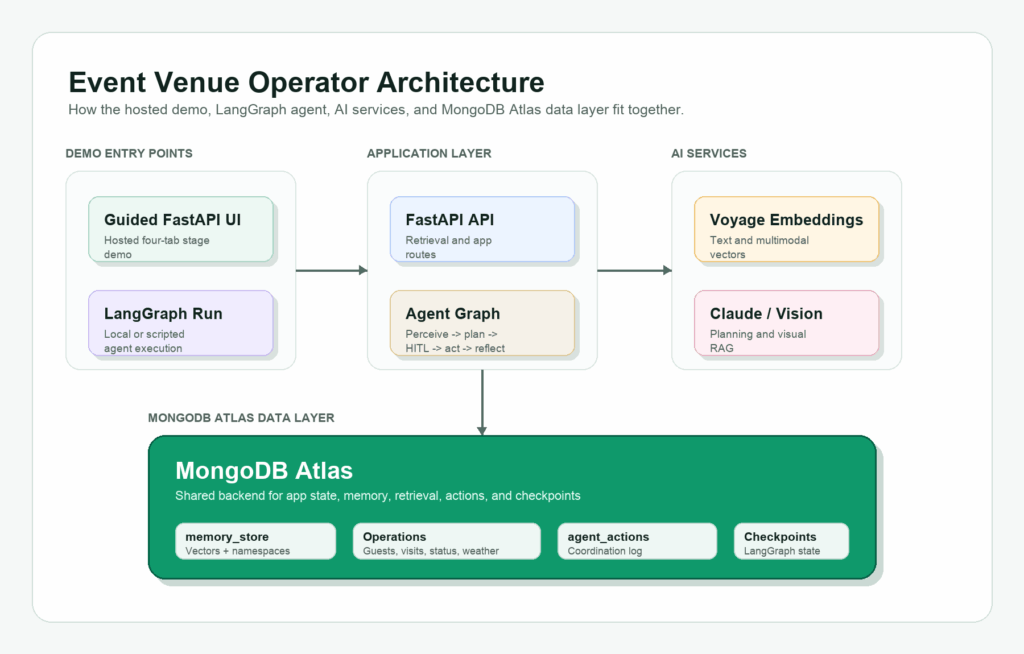
Introduction This tutorial starts where most agent demos stop: giving the agent persistent memory, operational context, and a place to write back what happened. An event operator does not just need an agent that can summarize a weather report or generate a generic plan. The operator needs an agent that can remember what happened at prior events, retrieve relevant visitor and venue context, respond to live operational changes, and write the outcome back as memory for the next similar situation. We built this event-venue operator demo with MongoDB Atlas, Voyage AI embeddings, LangGraph, and optional Langfuse tracing. The demo scenario is the MongoDB Open, a fictional premium tennis tournament on Day 6 of play. Rain is approaching, covered hospitality capacity is constrained, and the operator has two different visitor journeys to protect: Mikiko, a first-time attendee trying to make the most of the grounds, and Nina, a premier guest with hospitality expectations and a history the agent can retrieve. This is not a customer case study or a production deployment. It is a fictional builder scenario inspired by real event operations economics. Major tennis events show why these decisions matter: the 2025 US Open broke attendance, viewership, and digital reach records and offered $90 million in total player compensation; USTA has also said the three-week US Open drives more than $1.2 billion in annual economic impact for New York City. Premium fan expectations are high, too: PwC found that 60% of high-income U.S. sports fans would spend more than $250 for a special event, and 20% would spend more than $1,000. Weather adds another layer of risk, which is why the U.S. Census Bureau now tracks the monetary impact of extreme weather on business sales through its Business Trends and Outlook Survey. The MongoDB Open demo agent is not just producing a plausible plan. It reads current venue state, retrieves prior event memory, distinguishes between visitor segments, and acts. At the same time, hospitality capacity is still available, and writes the outcome back so the next disruption can be handled with more context. Check out the full repo here.  The demo is split into three layers: A guided, deterministic UI that makes the operator story easy to follow. A hosted Vercel demo that gives readers a public app link. Live API endpoints and scripts for Atlas Vector Search, vector-plus-lexical retrieval, visual-document RAG, LangGraph execution, and optional Langfuse traces, to demonstrate how the stack all works together.  What You Will Build By the end of the tutorial, you will have a FastAPI app backed by MongoDB Atlas that can run locally and deploy to Vercel. The app includes: A four-tab guided UI for the event-operations story and live backend validation. Atlas collections for operational state, semantic memory, agent actions, and LangGraph checkpoints. Voyage multimodal embeddings stored in Atlas. Atlas Vector Search for memory retrieval. A hybrid retrieval endpoint that combines vector similarity with lexical scoring. A Vision RAG endpoint that retrieves visual operational documents and passes them to Claude Vision. Optional Langfuse tracing for retrieval calls and the live LangGraph run. A runnable LangGraph script that follows the same rain-delay story. A Vercel deployment configuration for a hosted demo. The current repo should be treated as a reference demo, not a production platform. There is no production auth, no CI suite, and the full LangGraph agent remains a script-based validation path rather than a public hosted endpoint. Architecture Overview The architecture centers on MongoDB Atlas as both the operational and memory layer. Speed matters in the event venue operator scenario because the useful window for action is short. If rain is 20 minutes away and covered hospitality space is filling up, the operator does not need a post-event dashboard or a batch summary a few minutes later. The agent needs to read the current venue state, retrieve relevant memory, decide what to do, and write back the result while there is still capacity to protect the guest experience. That is why the type of database and how it is used are critical system design choices. Operational records, semantic memory, vector embeddings, visual documents, and agent actions all live in the same data layer. The agent does not need to wait for a separate analytics pipeline, sync data into a second vector database, or reconcile what the memory layer says with what the operational system says. Atlas acts as both the system of record and the retrieval layer for the agent loop: perceive what changed, retrieve the right context, take action, and persist what happened for the next event. This is also why the demo keeps memory in MongoDB rather than treating it as a sidecar. The agent is not just retrieving chunks; it is composing operational context. A useful decision may need visitor history, current venue status, hospitality inventory, prior rain-delay patterns, and relevant visual documents at the same time. With Atlas, those pieces can stay queryable together instead of being scattered across separate systems. Caption: MongoDB Atlas stores the demo’s operational state, semantic memory, visual document embeddings, agent actions, and LangGraph checkpoints in one backend. The demo uses four main state layers: Operational records: guests, visits, venue status, weather events, reservations, event metrics, and agent actions. Semantic memory: memory_store, with Voyage embeddings and Atlas Vector Search. Visual documents: operational images embedded into the same memory store as image-derived multimodal embeddings and document metadata. Agent state: LangGraph checkpoints and checkpoint writes. Setup Before you begin, make sure you have: Python 3.12 or later uv installed A MongoDB Atlas cluster with Vector Search enabled (this can be set up for free) An Anthropic API key (or feel free to use an LLM of your choice and reconfigure API keys) A Voyage API key (this can be set up for free) Clone the repo and install dependencies: GitHub repo Copy CodeCopiedUse a different Browser git clone https://github.com/mongodb-developer/event-venue-operator.git cd event-venue-operator uv sync If you only want to inspect the app before setting up credentials, start with the live Vercel demo. The hosted demo

Build an Agentic Event Venue Operator with MongoDB Atlas, Voyage, and LangGraph Read Post »

AI, Committee, ข่าว, Uncategorized

Google Cloud’s Always-On Memory Agent Replaces RAG and Embeddings With Continuous LLM Consolidation on Gemini 3.1 Flash-Lite

Most AI agents forget. They process a request, answer it, then drop the context. Google Cloud’s generative-ai repository now ships a sample that tackles this directly. It is the Always-On Memory Agent, a reference implementation that treats memory as a running process. Always-On Memory Agent Fundamentally, the project is a lightweight background agent that never stops. It runs 24/7 as a continuous process, not a one-shot call. It is built with Google ADK (Agent Development Kit) and Gemini 3.1 Flash-Lite. Notably, it uses no vector database and no embeddings. Instead, an LLM reads, thinks, and writes structured memory into SQLite. The model choice targets low latency and low cost for continuous background work. How It Works: Ingest, Consolidate, Query Architecturally, an orchestrator routes every request to one of three specialist sub-agents. Each sub-agent owns its own tools for reading or writing the memory store. First, the IngestAgent handles incoming content. It uses Gemini’s multimodal capabilities to extract a summary, entities, topics, and an importance score. That structured record then lands in the memories table. Next, the ConsolidateAgent runs on a timer, every 30 minutes by default. Like sleep cycles, it reviews unconsolidated memories and finds connections between them. Then it writes a synthesized summary, one key insight, and those connections to the database. Consequently, the agent builds new understanding while idle, with no prompt. Finally, the QueryAgent answers questions. It reads all memories and consolidation insights, then synthesizes a response. Importantly, it cites the memory IDs it used as sources. “, src:”report.pdf”, sm:”Anthropic reports 62% of Claude usage is code-related.”, ent:[“Anthropic”,”Claude”,”AI agents”], tp:[“AI”,”code generation”], imp:0.8}, {icon:”“, src:”roadmap.png”, sm:”Q1 priority: reduce inference costs by 40%.”, ent:[“Q1″,”inference”], tp:[“cost”,”planning”], imp:0.7}, {icon:”“, src:”standup.mp3″, sm:”AI agents grow fast, but reliability is still a challenge.”, ent:[“AI agents”,”reliability”], tp:[“agents”,”reliability”], imp:0.75}, {icon:”“, src:”idea.txt”, sm:”Smart inbox idea: persistent AI memory for email.”, ent:[“smart inbox”,”email”], tp:[“product”,”memory”], imp:0.6} ]; var CONS = { links:[[1,3],[2,1],[3,4]], insight:”The bottleneck for next-gen AI tools is the transition from static RAG to dynamic memory systems.” }; var Q = “What should I focus on?”; var A = ‘Based on your memories, prioritize: ship the cost-reduction plan <span class="”ref”">[Memory 2]</span>, ‘ + ‘then close the agent reliability gap <span class="”ref”">[Memory 3]</span>. ‘ + ‘The smart inbox concept <span class="”ref”">[Memory 4]</span> validates demand for persistent AI memory.’; var i=0, consolidated=false; var $=function(id){return document.getElementById(id)}; var store=$(“store”), pkt=$(“pkt”), logEl=$(“log”); function post(){ try{ parent.postMessage({type:”aoma-resize”,height:document.body.offsetHeight+40},”*”); }catch(e){} } function log(html){ logEl.innerHTML=html; post(); } function activate(el,cls){ [ “sIngest”,”sCons”,”sQuery” ].forEach(function(id){ $(id).classList.remove(“active”,”cons”,”query”); }); if(el){ el.classList.add(“active”); if(cls) el.classList.add(cls); } } function packet(color){ pkt.style.background=color; pkt.style.opacity=”1″; pkt.style.left=”0″; setTimeout(function(){ pkt.style.left=”calc(100% – 10px)”; },30); setTimeout(function(){ pkt.style.opacity=”0″; },950); } function ingest(){ if(i>=SAMPLES.length){ log(“<b>Inbox empty.</b> All 4 sample files ingested — now consolidate or query.”); return; } var s=SAMPLES[i]; var id=i+1; activate($(“sIngest”)); packet(“#4285F4”); log(‘<b>IngestAgent</b> reads <b>’+s.icon+’ ‘+s.src+'</b> → extracting summary, entities, topics, importance…’); var c=document.createElement(“div”); c.className=”card”; c.id=”card”+id; c.innerHTML='<span class="”cid”">#’+id+'</span><div class="”sm”">’+s.sm+'</div>’+ ‘<div class="”chips”">’+s.ent.map(function(e){return ‘<span class="”chip”">’+e+'</span>’}).join(“”)+'</div>’+ ‘<div class="”chips”">’+s.tp.map(function(t){return ‘<span class="”chip" tp”>’+t+'</span>’}).join(“”)+'</div>’+ ‘<div class="”imp”">importance <b>’+s.imp+'</b></div>’; store.appendChild(c); post(); setTimeout(function(){ c.classList.add(“show”); post(); log(‘<b>Stored memory #’+id+'</b> in SQLite. ‘+(SAMPLES.length-id)+’ file(s) left in inbox.’); },500); i++; if(i>=2){ $(“bCons”).disabled=false; $(“bQuery”).disabled=false; } } function consolidate(){ if(i<2){ log(“Ingest at least 2 memories first.”); return; } activate($(“sCons”),”cons”); packet(“#FBBC04”); $(“tmr”).classList.add(“run”); log(“<b>ConsolidateAgent</b> woke on its 30-min timer — reviewing unconsolidated memories…”); var svg=$(“wires”); svg.innerHTML=””; for(var k=1;k<=Math.min(i,4);k++){ var el=$(“card”+k); if(el) el.classList.add(“hl”); } setTimeout(function(){ CONS.links.forEach(function(pair){ drawWire(pair[0],pair[1]); }); log(“<b>Found connections</b> across memories — writing one cross-cutting insight…”); },500); setTimeout(function(){ var ins=$(“insight”); ins.innerHTML='<b>Insight:</b> ‘+CONS.insight; ins.classList.add(“show”); $(“tmr”).classList.remove(“run”); consolidated=true; log(“<b>Consolidation done.</b> New insight written back to the store — no prompt needed.”); post(); },1200); } function drawWire(a,b){ var svg=$(“wires”), ca=$(“card”+a), cb=$(“card”+b); if(!ca||!cb) return; var box=svg.getBoundingClientRect(), ra=ca.getBoundingClientRect(), rb=cb.getBoundingClientRect(); var x1=ra.left-box.left+ra.width/2, y1=ra.top-box.top+ra.height/2; var x2=rb.left-box.left+rb.width/2, y2=rb.top-box.top+rb.height/2; var ln=document.createElementNS(“http://www.w3.org/2000/svg”,”line”); ln.setAttribute(“x1”,x1);ln.setAttribute(“y1”,y1);ln.setAttribute(“x2”,x1);ln.setAttribute(“y2”,y1); ln.setAttribute(“stroke”,”#FBBC04″);ln.setAttribute(“stroke-width”,”2″);ln.setAttribute(“stroke-dasharray”,”4 3″); svg.appendChild(ln); requestAnimationFrame(function(){ ln.style.transition=”all .5s”; ln.setAttribute(“x2”,x2); ln.setAttribute(“y2”,y2); }); } function query(){ if(i<1){ log(“Ingest something first.”); return; } activate($(“sQuery”),”query”); packet(“#34A853”); $(“qbox”).classList.add(“show”); $(“qask”).textContent=’Q: ‘+Q; $(“qans”).innerHTML=”Reading all memories…”; log(“<b>QueryAgent</b> reads every memory”+(consolidated?” and the consolidation insight”:””)+”, then synthesizes…”); [“card2″,”card3″,”card4”].forEach(function(id){ var el=$(id); if(el) el.classList.add(“cite”); }); setTimeout(function(){ $(“qans”).innerHTML=A; log(“<b>Answer returned</b> with cited memory IDs — grounded only in stored memories.”); post(); },900); } function reset(){ i=0; consolidated=false; store.innerHTML=””; $(“wires”).innerHTML=””; $(“insight”).className=”insight”; $(“insight”).innerHTML=””; $(“qbox”).className=”qbox”; $(“qans”).innerHTML=””; $(“qask”).textContent=””; $(“bCons”).disabled=true; $(“bQuery”).disabled=true; activate(null); log(“<b>Reset.</b> Drop a file into the agent’s inbox to begin.”); } $(“bIngest”).onclick=ingest; $(“bCons”).onclick=consolidate; $(“bQuery”).onclick=query; $(“bReset”).onclick=reset; window.addEventListener(“load”,post); window.addEventListener(“resize”,post); if(window.ResizeObserver){ new ResizeObserver(post).observe(document.body); } setTimeout(post,150); })(); </script> </body> </html> “> Supported Inputs Beyond text, the IngestAgent accepts 27 file types across five categories. Simply drop any supported file into the ./inbox folder for automatic pickup. Category Extensions Text .txt, .md, .json, .csv, .log, .xml, .yaml, .yml Images .png, .jpg, .jpeg, .gif, .webp, .bmp, .svg Audio .mp3, .wav, .ogg, .flac, .m4a, .aac Video .mp4, .webm, .mov, .avi, .mkv Documents .pdf How It Compares to RAG, Summaries, and Knowledge Graphs To clarify the difference, it frames three common memory approaches. Each solves part of the problem, yet leaves a gap. Approach How it stores Active processing Main limitation Vector DB + RAG Embeddings in a vector store None Passive; embeds once, retrieves later Conversation summary Compressed text None Loses detail; no cross-reference Knowledge graphs Nodes and edges Manual upkeep Expensive to build and maintain Always-On Memory Agent Structured rows in SQLite Continuous consolidation Query reads up to 50 recent memories Unlike RAG, this agent processes memory actively, not only on retrieval. Use Cases With Examples Practically, the pattern fits any workload needing durable, evolving context. Consider three examples. A research assistant ingests PDFs, meeting audio, and screenshots all week. Later, it links a cost target to a reliability problem on its own. A personal knowledge base absorbs notes, articles, and images continuously. Over time, consolidation surfaces themes you never explicitly connected. A support agent stores past tickets as structured memories. Then it answers new questions with cited references to earlier cases. Getting Started With the design clear, setup stays minimal for early-level engineers. Install dependencies, set your key, then start the process. Copy CodeCopiedUse a different Browser pip install -r requirements.txt export GOOGLE_API_KEY=”your-gemini-api-key” python agent.py Once running, the agent watches ./inbox, consolidates every 30 minutes, and serves an HTTP API on port 8888. Therefore, you can also feed it over HTTP. Copy CodeCopiedUse a different Browser #

Google Cloud’s Always-On Memory Agent Replaces RAG and Embeddings With Continuous LLM Consolidation on Gemini 3.1 Flash-Lite Read Post »

AI, Committee, ข่าว, Uncategorized

NVIDIA Released DeepStream 9.1: Bringing Agentic AI to Vision AI With 13 Skills and Multi-View 3D Tracking

NVIDIA just released DeepStream 9.1. The update targets a persistent problem in video analytics. Tracking one object across many cameras traditionally requires manual camera calibration and complicated calculations. DeepStream 9.1 addresses this with two additions: Multi-View 3D Tracking (MV3DT) and AutoMagicCalib (AMC). Both ship as agentic skills for coding agents. As a result, developers move from concept to a running pipeline faster. What is DeepStream 9.1 To understand the update, start with the base platform. DeepStream is NVIDIA’s streaming analytics toolkit for AI-based video and image understanding. It provides a GStreamer-based framework for multi-stream, multi-model inference on NVIDIA GPUs. Pipelines combine hardware-accelerated decoding and encoding, TensorRT inference, object tracking, and message-broker integration. Building on that base, version 9.1 adds five notable items: 13 agentic skills for coding agents. The MV3DT skill for cross-camera tracking. The AMC skill for automatic calibration. NVIDIA JetPack 7.2 support for Jetson Orin and Thor edge devices. A unified open-source GitHub repository under CC-BY-4.0 AND Apache-2.0. How MV3DT Tracks Objects Across Cameras Among those additions, MV3DT is the main skill, so consider how it works. At its core, MV3DT projects detections from multiple calibrated cameras into a shared 3D coordinate system. It then associates observations of the same object across camera views. Finally, it assigns one globally consistent object ID. Concretely, the data flow runs in four stages. For detection, each camera stream runs an object detector. MV3DT supports three models out of the box: PeopleNetTransformer: a transformer-based people detector, the default for pedestrian scenes. PeopleNet v2.6.3: a high-efficiency detector based on the DetectNet_v2 architecture. RT-DETR 2D: a multi-class detector for pedestrians, transporters, and forklifts. Next, for monocular 3D perception, each camera uses a 3×4 projection matrix stored in a YAML calibration file. This back-projects 2D bounding boxes into 3D world-space coordinates using a ground-plane assumption. Then, for multi-view association, the tracker shares tracklets using Message Queuing Telemetry Transport (MQTT). MQTT is a lightweight pub/sub messaging protocol. When two cameras observe the same person, it matches tracklets by proximity in 3D world space. After association, results stream out in three forms. The On-Screen Display (OSD) shows a tiled grid with 2D and 3D bounding boxes. The Bird’s-Eye View (BEV) renders a top-down trajectory map. Kafka messaging delivers per-frame protobuf metadata, including sensor ID, object ID, and 3D bounding box. How AutoMagicCalib Removes Manual Setup MV3DT depends on calibrated cameras, which traditionally means checkerboards and downtime. Instead, AMC calibrates a network by analyzing tracked objects in existing video files or streams. It estimates each camera’s intrinsic parameters (focal length, principal point, lens distortion). It also estimates extrinsic parameters (rotation, translation, world position). Under the hood, the pipeline runs five stages. These are per-camera trajectory extraction, single-view rectification, multi-view tracklet matching, bundle adjustment, and optional VGGT refinement. VGGT (Visual Geometry Grounded Transformer) helps when object movement is limited. AMC runs as a microservice with REST APIs and a web interface. Users supply only a layout image and a few alignment points. The Agentic Skills Workflow With MV3DT and AMC defined, the delivery mechanism is the skills themselves. Rather than editing configuration files, you describe intent in natural language. The skills work with Claude Code, Codex, Cursor, and similar agents. Setup is short: Copy CodeCopiedUse a different Browser git clone https://github.com/NVIDIA/DeepStream.git cd DeepStream # Copy skills into your agent’s skill directory (Codex shown) mkdir -p ~/.codex/skills cp -r skills/* ~/.codex/skills/ After launching the agent, a single prompt runs the reference app: Copy CodeCopiedUse a different Browser deploy mv3dt on the 12-camera sample dataset From there, the MV3DT skill validates prerequisites, pulls the container, and installs Kafka and Mosquitto broker services. It also downloads model weights, generates the pipeline config, and launches tracking. Notably, if calibration files are missing, it triggers the AMC skills automatically. DeepStream 9.0 vs 9.1 For context, the table below shows what changed between releases. Capability DeepStream 9.0 DeepStream 9.1 Agentic skills 2 (deepstream-dev, import-vision-model) 13 agentic skills Multi-camera 3D tracking Not shipped as a skill MV3DT skill + reference app Camera calibration Manual AutoMagicCalib (AMC) microservice Jetson support JetPack 7.1 GA JetPack 7.2 (Orin, Thor) Sample datasets — 4-camera and 12-camera MV3DT sets Distribution NGC packages + GitHub source Unified GitHub monorepo Use Cases With Examples Given these capabilities, the features map to concrete deployments: Warehouse safety: track a worker near forklifts across aisles with one ID, using RT-DETR 2D. Retail analytics: follow a shopper between camera zones to measure dwell time without re-identification errors. Smart-building monitoring: count occupancy across floors and feed Kafka metadata to dashboards. Robotics and smart cities: share consistent world coordinates for navigation and incident review. Interactive Explainer To see the mechanism, the embedded demo below animates one person walking between three camera fields of view. Toggle between naive per-camera 2D tracking and MV3DT 3D fusion to watch the object ID stay consistent. Key Takeaways DeepStream 9.1 ships 13 agentic skills, letting coding agents build multi-camera vision pipelines from natural-language prompts. MV3DT fuses per-camera detections into one shared 3D world, keeping a single globally consistent object ID across views. AutoMagicCalib replaces manual checkerboard calibration by estimating camera intrinsics and extrinsics from existing video. JetPack 7.2 support extends deployment to Jetson Orin and Thor, under a unified open-source GitHub monorepo. Outputs stream as OSD, Bird’s-Eye View, and Kafka protobuf metadata, ready for downstream analytics and dashboards. Check out the Repo here. Also, feel free to follow us on Twitter and don’t forget to join our 150k+ML SubReddit and Subscribe to our Newsletter. Wait! are you on telegram? now you can join us on telegram as well. Need to partner with us for promoting your GitHub Repo OR Hugging Face Page OR Product Release OR Webinar etc.? Connect with us The post NVIDIA Released DeepStream 9.1: Bringing Agentic AI to Vision AI With 13 Skills and Multi-View 3D Tracking appeared first on MarkTechPost.

NVIDIA Released DeepStream 9.1: Bringing Agentic AI to Vision AI With 13 Skills and Multi-View 3D Tracking Read Post »

AI, Committee, ข่าว, Uncategorized

NVIDIA AI Releases Nemotron 3 Embed: An Open Embedding Collection Whose 8B Checkpoint Ranks #1 on RTEB

Embedding models decide which passages an agent ever sees. NVIDIA released Nemotron 3 Embed model to work on that layer. It targets production-scale RAG, agentic retrieval, code retrieval, and agent memory. What is Nemotron 3 Embed? The model collection includes three open checkpoints. Nemotron-3-Embed-8B-BF16 is the accuracy-first option. Nemotron-3-Embed-1B-BF16 carries the same design into a smaller footprint. Nemotron-3-Embed-1B-NVFP4 is the Blackwell-optimized 4-bit path. All three are transformer encoders trained with bidirectional attention masking. The final embedding comes from average pooling over token-level representations. Maximum sequence length is 32,768 tokens on every checkpoint. Each model was evaluated across 34 languages. All three carry the OpenMDW License Agreement, version 1.1 (OpenMDW-1.1). Notably, the bases are Mistral models. The 8B is built with Ministral-3-8B-Instruct-2512. Both 1B variants use Ministral-3-3B-Instruct-2512. Performance Nemotron-3-Embed-8B-BF16 ranks #1 overall on RTEB (as of July 17 2026), the Retrieval Embedding Benchmark. Evaluation covers its 16 public tasks. Every figure below is average NDCG@10, at model sequence length 4096. Model Params Emb dim RTEB ViDoRe-V3 text MMTEB (Retrieval) Nemotron-3-Embed-8B-BF16 ~8B 4096 78.46 60.60 75.45 Nemotron-3-Embed-1B-BF16 1.14B 2048 72.38 57.74 71.04 Nemotron-3-Embed-1B-NVFP4 1.14B 2048 72.00 — — llama-nemotron-embed-vl-1b-v2 — — 61.98 52.54 59.71 llama-nemotron-embed-1b-v2 — — 60.47 52.10 59.58 Two gaps are worth noting. The 1B gains 10.4 RTEB points over llama-nemotron-embed-vl-1b-v2, the prior-generation baseline. Separately, NVFP4 costs 0.38 RTEB points against its BF16 parent, or 99.5% retention. How the 1B Model was Built? Those 1B scores come from a compression pipeline, not a smaller training run. The parent was nemotron-3-embed-3b, pruned and distilled across two iterative rounds. First, the 3B parent was pruned to 2B using NVIDIA ModelOpt mcore_minitron Neural Architecture Search (NAS). The search covers hidden width, FFN size, attention heads, and depth. It then picks the best candidate from the top-10 Pareto front. A 50k in-domain calibration corpus scored those candidates. Next, the 2B model was distilled from the fine-tuned 8B embedding teacher. Distillation combined cosine distance loss (COS) and mean squared error (MSE) loss. The data blend was multilingual and in-domain. Finally, the same procedure repeated to produce the 1.14B checkpoint. The NVFP4 Serving Tradeoff Compression then continues into the serving format. Quantization hit weights and activations of linear layers only, targeting the NVFP4 data type. The research team used nvidia-modelopt v0.45.0. Quantization-Aware Distillation (QAD) followed, primarily to recover accuracy on long inputs. Calibration used 512 samples: 256 queries and 256 passages from abisee/cnn_dailymail. QAD training used 20k samples. The rsesearch team reports NVFP4 on Blackwell delivers up to 2x higher throughput than BF16. It retains 99%+ of BF16 retrieval accuracy. The NVFP4 card also documents dynamic embedding sizes. You can slice the 2048-d vector from the start to 1024 or 512 dimensions. Re-normalize afterward. Interactive Explainer: The Five-Stage Retrieval Path Before touching code, watch the path run. It animates prefixing, bidirectional encoding, average pooling, L2 normalization, and dot-product scoring. Scores come from each card’s published expected output. Deployment Matrix As that walkthrough implies, the checkpoints do not share runtime paths. Feature 8B-BF16 1B-BF16 1B-NVFP4 Transformers / Sentence Transformers Yes Yes No vLLM for /v2/embed 0.25.0 0.25.0 0.25.0 Microarchitectures Ampere, Hopper, Blackwell Ampere, Hopper, Blackwell Ampere, Hopper, Lovelace, Blackwell Test hardware A100 80GB, H100 80GB A100 80GB, H100 80GB GB200, RTX 6000 PRO, A100, H100, L40, L4 Training data 50M+ samples 8.5M+ (distillation) 20k (QAD) Alongside the checkpoints, NVIDIA research team released an optimized NIM microservice for the 1B model. The Rust-based NIM matches or outperforms the vLLM checkpoint on GB200 and RTX PRO 6000. NVIDIA tested input sequence lengths of 256 and 1024. Separately, NVIDIA NeMo AutoModel recipes cover fine-tuning and distillation. Using It in Code With those paths in mind, prefixes come first. Queries take query: and documents take passage: . Embeddings are L2-normalized, so dot product equals cosine similarity. Copy CodeCopiedUse a different Browser # pip install –upgrade “transformers>=5.2.0” “sentence-transformers>=5.4.1” import torch from sentence_transformers import SentenceTransformer QUERIES = [“How can someone reduce exposure to pollen during allergy season?”] DOCUMENTS = [“People with pollen allergy can reduce exposure by staying indoors ” “on dry, windy days, avoiding early-morning outdoor activity, and ” “going outside after rain when pollen levels are lower.”] model = SentenceTransformer( “nvidia/Nemotron-3-Embed-8B-BF16″, device=”cuda”, model_kwargs={“dtype”: torch.bfloat16, # use “sdpa” if FlashAttention-2 is unavailable “attn_implementation”: “flash_attention_2”}, processor_kwargs={“padding_side”: “left”}, ) model.max_seq_length = 32768 q = model.encode_query(QUERIES, batch_size=1, convert_to_tensor=True) d = model.encode_document(DOCUMENTS, batch_size=1, convert_to_tensor=True) print(model.similarity(q, d)) # card’s published q[3]/d[3] score: 0.8008 encode_query and encode_document read the saved prompts. So you never add prefixes by hand. For serving, /v2/embed applies them from input_type instead: Copy CodeCopiedUse a different Browser vllm serve nvidia/Nemotron-3-Embed-1B-NVFP4 –max-model-len 4096 –max-num-batched-tokens 4096 –max-cudagraph-capture-size 4096 Copy CodeCopiedUse a different Browser import numpy as np, requests def embed(input_type: str, texts: list[str]) -> np.ndarray: r = requests.post( “http://localhost:8000/v2/embed”, json={“model”: “nvidia/Nemotron-3-Embed-1B-NVFP4”, “input_type”: input_type, # “query” or “document” “texts”: texts, “embedding_types”: [“float”], “truncate”: “END”}, timeout=120, ) r.raise_for_status() return np.array(r.json()[“embeddings”][“float”], dtype=np.float32) scores = embed(“query”, QUERIES) @ embed(“document”, DOCUMENTS).T Use Cases With Examples Multilingual enterprise search: A support team indexes Hindi, Japanese, and English tickets together. Because retrieval is cross-lingual, a German query can surface a Japanese resolution note. Code retrieval: Training included coir_apps, coir_cosqa, synthetic_text2sql, and SWE-bench. Natural-language-to-code lookup is therefore closer to in-distribution. Agent memory: The 32,768-token limit lets an agent embed long conversation summaries without aggressive chunking. Cost-tiered RAG: Serve 1B-NVFP4 for high-volume recall, and route hard queries to the 8B. Because widths differ, this needs two indexes. Key Takeaways Nemotron-3-Embed-8B-BF16 ranks #1 on RTEB at 78.46 avg NDCG@10. Three open checkpoints span 8B BF16, 1B BF16, and 1B NVFP4. NVFP4 retains 99%+ of BF16 accuracy at up to 2x Blackwell throughput. The 1B came from ModelOpt NAS pruning plus COS+MSE distillation from the 8B. All checkpoints use OpenMDW-1.1 and support 32,768-token inputs. Check out the NVIDIA launch post on Hugging Face, Nemotron 3 Embed collection, 8B-BF16 card, 1B-BF16 card and 1B-NVFP4 card. Also, feel free to follow us on Twitter and don’t forget to join our 150k+ML SubReddit and Subscribe to our Newsletter. Wait! are you on telegram? now you can join us on telegram as well. Need to partner with us for

NVIDIA AI Releases Nemotron 3 Embed: An Open Embedding Collection Whose 8B Checkpoint Ranks #1 on RTEB Read Post »

We use cookies to improve your experience and performance on our website. You can learn more at นโยบายความเป็นส่วนตัว and manage your privacy settings by clicking Settings.

ตั้งค่าความเป็นส่วนตัว

You can choose your cookie settings by turning on/off each type of cookie as you wish, except for essential cookies.

ยอมรับทั้งหมด
จัดการความเป็นส่วนตัว
  • เปิดใช้งานตลอด

บันทึกการตั้งค่า
th