A deep neural network can be understood as a geometric system, where each layer reshapes the input space to form increasingly complex decision boundaries. For this to work effectively, layers must preserve meaningful spatial information — particularly how far a data point lies from these boundaries — since this distance enables deeper layers to build rich, non-linear representations. Sigmoid disrupts this process by compressing all inputs into a narrow range between 0 and 1. As values move away from decision boundaries, they become indistinguishable, causing a loss of geometric context across layers. This leads to weaker representations and limits the effectiveness of depth. ReLU, on the other hand, preserves magnitude for positive inputs, allowing distance information to flow through the network. This enables deeper models to remain expressive without requiring excessive width or compute. In this article, we focus on this forward-pass behavior — analyzing how Sigmoid and ReLU differ in signal propagation and representation geometry using a two-moons experiment, and what that means for inference efficiency and scalability. Setting up the dependencies Copy CodeCopiedUse a different Browser import numpy as np import matplotlib.pyplot as plt import matplotlib.gridspec as gridspec from matplotlib.colors import ListedColormap from sklearn.datasets import make_moons from sklearn.preprocessing import StandardScaler from sklearn.model_selection import train_test_split Copy CodeCopiedUse a different Browser plt.rcParams.update({ “font.family”: “monospace”, “axes.spines.top”: False, “axes.spines.right”: False, “figure.facecolor”: “white”, “axes.facecolor”: “#f7f7f7”, “axes.grid”: True, “grid.color”: “#e0e0e0”, “grid.linewidth”: 0.6, }) T = { “bg”: “white”, “panel”: “#f7f7f7”, “sig”: “#e05c5c”, “relu”: “#3a7bd5”, “c0”: “#f4a261”, “c1”: “#2a9d8f”, “text”: “#1a1a1a”, “muted”: “#666666”, } Creating the dataset To study the effect of activation functions in a controlled setting, we first generate a synthetic dataset using scikit-learn’s make_moons. This creates a non-linear, two-class problem where simple linear boundaries fail, making it ideal for testing how well neural networks learn complex decision surfaces. We add a small amount of noise to make the task more realistic, then standardize the features using StandardScaler so both dimensions are on the same scale — ensuring stable training. The dataset is then split into training and test sets to evaluate generalization. Finally, we visualize the data distribution. This plot serves as the baseline geometry that both Sigmoid and ReLU networks will attempt to model, allowing us to later compare how each activation function transforms this space across layers. Copy CodeCopiedUse a different Browser X, y = make_moons(n_samples=400, noise=0.18, random_state=42) X = StandardScaler().fit_transform(X) X_train, X_test, y_train, y_test = train_test_split( X, y, test_size=0.25, random_state=42 ) fig, ax = plt.subplots(figsize=(7, 5)) fig.patch.set_facecolor(T[“bg”]) ax.set_facecolor(T[“panel”]) ax.scatter(X[y == 0, 0], X[y == 0, 1], c=T[“c0″], s=40, edgecolors=”white”, linewidths=0.5, label=”Class 0″, alpha=0.9) ax.scatter(X[y == 1, 0], X[y == 1, 1], c=T[“c1″], s=40, edgecolors=”white”, linewidths=0.5, label=”Class 1″, alpha=0.9) ax.set_title(“make_moons — our dataset”, color=T[“text”], fontsize=13) ax.set_xlabel(“x₁”, color=T[“muted”]); ax.set_ylabel(“x₂”, color=T[“muted”]) ax.tick_params(colors=T[“muted”]); ax.legend(fontsize=10) plt.tight_layout() plt.savefig(“moons_dataset.png”, dpi=140, bbox_inches=”tight”) plt.show() Creating the Network Next, we implement a small, controlled neural network to isolate the effect of activation functions. The goal here is not to build a highly optimized model, but to create a clean experimental setup where Sigmoid and ReLU can be compared under identical conditions. We define both activation functions (Sigmoid and ReLU) along with their derivatives, and use binary cross-entropy as the loss since this is a binary classification task. The TwoLayerNet class represents a simple 3-layer feedforward network (2 hidden layers + output), where the only configurable component is the activation function. A key detail is the initialization strategy: we use He initialization for ReLU and Xavier initialization for Sigmoid, ensuring that each network starts in a fair and stable regime based on its activation dynamics. The forward pass computes activations layer by layer, while the backward pass performs standard gradient descent updates. Importantly, we also include diagnostic methods like get_hidden and get_z_trace, which allow us to inspect how signals evolve across layers — this is crucial for analyzing how much geometric information is preserved or lost. By keeping architecture, data, and training setup constant, this implementation ensures that any difference in performance or internal representations can be directly attributed to the activation function itself — setting the stage for a clear comparison of their impact on signal propagation and expressiveness. Copy CodeCopiedUse a different Browser def sigmoid(z): return 1 / (1 + np.exp(-np.clip(z, -500, 500))) def sigmoid_d(a): return a * (1 – a) def relu(z): return np.maximum(0, z) def relu_d(z): return (z > 0).astype(float) def bce(y, yhat): return -np.mean(y * np.log(yhat + 1e-9) + (1 – y) * np.log(1 – yhat + 1e-9)) class TwoLayerNet: def __init__(self, activation=”relu”, seed=0): np.random.seed(seed) self.act_name = activation self.act = relu if activation == “relu” else sigmoid self.dact = relu_d if activation == “relu” else sigmoid_d # He init for ReLU, Xavier for Sigmoid scale = lambda fan_in: np.sqrt(2 / fan_in) if activation == “relu” else np.sqrt(1 / fan_in) self.W1 = np.random.randn(2, 8) * scale(2) self.b1 = np.zeros((1, 8)) self.W2 = np.random.randn(8, 8) * scale(8) self.b2 = np.zeros((1, 8)) self.W3 = np.random.randn(8, 1) * scale(8) self.b3 = np.zeros((1, 1)) self.loss_history = [] def forward(self, X, store=False): z1 = X @ self.W1 + self.b1; a1 = self.act(z1) z2 = a1 @ self.W2 + self.b2; a2 = self.act(z2) z3 = a2 @ self.W3 + self.b3; out = sigmoid(z3) if store: self._cache = (X, z1, a1, z2, a2, z3, out) return out def backward(self, lr=0.05): X, z1, a1, z2, a2, z3, out = self._cache n = X.shape[0] dout = (out – self.y_cache) / n dW3 = a2.T @ dout; db3 = dout.sum(axis=0, keepdims=True) da2 = dout @ self.W3.T dz2 = da2 * (self.dact(z2) if self.act_name == “relu” else self.dact(a2)) dW2 = a1.T @ dz2; db2 = dz2.sum(axis=0, keepdims=True) da1 = dz2 @ self.W2.T dz1 = da1 * (self.dact(z1) if self.act_name == “relu” else self.dact(a1)) dW1 = X.T @ dz1; db1 = dz1.sum(axis=0, keepdims=True) for p, g in [(self.W3,dW3),(self.b3,db3),(self.W2,dW2), (self.b2,db2),(self.W1,dW1),(self.b1,db1)]: p -= lr * g def train_step(self, X, y, lr=0.05): self.y_cache = y.reshape(-1, 1) out = self.forward(X, store=True) loss = bce(self.y_cache, out) self.backward(lr) return loss def get_hidden(self, X, layer=1): “””Return post-activation values for layer 1 or 2.””” z1 = X @ self.W1 + self.b1; a1 = self.act(z1) if