YouZum

Uncategorized

AI, Committee, Notizie, Uncategorized

Task-Lens: Cross-Task Utility Based Speech Dataset Profiling for Low-Resource Indian Languages

arXiv:2602.23388v1 Announce Type: new Abstract: The rising demand for inclusive speech technologies amplifies the need for multilingual datasets for Natural Language Processing (NLP) research. However, limited awareness of existing task-specific resources in low-resource languages hinders research. This challenge is especially acute in linguistically diverse countries, such as India. Cross-task profiling of existing Indian speech datasets can alleviate the data scarcity challenge. This involves investigating the utility of datasets across multiple downstream tasks rather than focusing on a single task. Prior surveys typically catalogue datasets for a single task, leaving comprehensive cross-task profiling as an open opportunity. Therefore, we propose Task-Lens, a cross-task survey that assesses the readiness of 50 Indian speech datasets spanning 26 languages for nine downstream speech tasks. First, we analyze which datasets contain metadata and properties suitable for specific tasks. Next, we propose task-aligned enhancements to unlock datasets to their full downstream potential. Finally, we identify tasks and Indian languages that are critically underserved by current resources. Our findings reveal that many Indian speech datasets contain untapped metadata that can support multiple downstream tasks. By uncovering cross-task linkages and gaps, Task-Lens enables researchers to explore the broader applicability of existing datasets and to prioritize dataset creation for underserved tasks and languages.

Task-Lens: Cross-Task Utility Based Speech Dataset Profiling for Low-Resource Indian Languages Leggi l'articolo »

AI, Committee, Notizie, Uncategorized

FireRedTeam Releases FireRed-OCR-2B Utilizing GRPO to Solve Structural Hallucinations in Tables and LaTeX for Software Developers

Document digitization has long been a multi-stage problem: first detect the layout, then extract the text, and finally try to reconstruct the structure. For Large Vision-Language Models (LVLMs), this often leads to ‘structural hallucinations’—disordered rows, invented formulas, or unclosed syntax. The FireRedTeam has released FireRed-OCR-2B, a flagship model designed to treat document parsing as a structural engineering task rather than ‘impressionist’ text generation. Built on the Qwen3-VL-2B-Instruct architecture, this model establishes a new State-of-the-Art (SOTA) for end-to-end solutions, achieving an overall score of 92.94% on the OmniDocBench v1.5 benchmark. Shifting the Paradigm: Structural Engineering vs. Text Generation Devs often find that even the most powerful general VLMs struggle with the dense spatial logic of a technical PDF. When a model ‘sees’ a complex table or a multi-line LaTeX equation, it frequently fails to maintain the hierarchical relationship between elements. FireRed-OCR-2B addresses this through a specialized Progressive Training Pipeline consisting of three distinct stages: Multi-task Pre-alignment: This stage establishes spatial grounding by training the model on detection, region recognition, and layout-to-markdown tasks. Specialized SFT (Supervised Fine-Tuning): The model is fine-tuned on a high-quality, standardized Markdown dataset to ensure logical consistency and hierarchical expression. Format-Constrained GRPO: The final stage uses reinforcement learning to enforce syntactic validity. The Core Innovation: Format-Constrained GRPO The most significant technical differentiator for FireRed-OCR is its use of Format-Constrained Group Relative Policy Optimization (GRPO). While traditional fine-tuning focuses on character accuracy, GRPO introduces a reinforcement learning loop that rewards the model for specific structural traits: Formula Syntax: Ensuring LaTeX equations are mathematically valid. Table Integrity: Maintaining consistent row/column counts and proper HTML/Markdown tagging. Hierarchical Closure: Verifying that all opened structural tags (like lists or headers) are correctly closed. Text Accuracy: Reducing character-level errors in dense text blocks. By eliminating the need for a separate ‘critic’ model—a key benefit of the GRPO algorithm—FireRedTeam has optimized the training process to focus specifically on the high-friction areas of document parsing. Solving the Long-Tail Layout Problem The ‘long-tail’ of document layouts (e.g., non-standard legal forms, academic papers with overlapping figures, or handwritten annotations) is where most OCR pipelines break. FireRed-OCR utilizes a ‘Geometry + Semantics’ Data Factory. This novel approach uses geometric feature clustering and multi-dimensional tagging to synthesize balanced datasets. By combining geometric awareness with semantic understanding, the model maintains ‘In-the-Wild Robustness,’ outperforming traditional pipeline systems like PaddleOCR on complex, non-standard layouts (benchmarked on the FireRedBench dataset). Performance Benchmarks In head-to-head comparisons on OmniDocBench v1.5, FireRed-OCR-2B (92.94%) significantly outperforms other end-to-end models, including: DeepSeek-OCR 2: 91.09% Gemini-3.0 Pro: 90.33% Qwen3-VL-235B: 89.15% While some ‘pipeline’ solutions (which use separate models for detection and recognition) achieve slightly higher scores, FireRed-OCR-2B represents the leading performance for a single-model, end-to-end approach. This is particularly relevant for devs looking to reduce system complexity and inference latency in production RAG (Retrieval-Augmented Generation) environments. Key Takeaways I have summarized the technical significance and performance metrics of the FireRed-OCR-2B release into five key takeaways for AI engineers and data scientists. 5 Key Takeaways: FireRed-OCR-2B New End-to-End SOTA Performance: FireRed-OCR-2B has achieved a state-of-the-art (SOTA) score of 92.94% on the OmniDocBench v1.5 benchmark. This makes it the leading single-model solution for document parsing, outperforming significantly larger models like Qwen2-VL-72B and Gemini-1.5-Pro in structural accuracy. Architectural Foundation: Built on the Qwen2-VL-2B-Instruct (or the updated 2026 iteration) base, the model utilizes a Vision-Language-Model (VLM) approach. It replaces traditional multi-stage pipelines (separate detection, cropping, and OCR steps) with a unified, end-to-end transformer architecture that outputs structured Markdown directly. Structural Integrity via GRPO: A major technical differentiator is the use of Format-Constrained GRPO (Group Relative Policy Optimization). This reinforcement learning technique rewards the model for maintaining syntactic validity—specifically ensuring that LaTeX formulas, table tags, and Markdown hierarchies are logically closed and mathematically consistent. ‘Geometry + Semantics’ Data Factory: To solve the problem of complex ‘in-the-wild’ layouts, the FireRedTeam developed a specialized data engine. This ‘factory’ synthesizes datasets by balancing geometric layout features with semantic content, enabling the model to handle overlapping figures, multi-column academic papers, and non-standard forms more reliably than previous iterations. Check out the Model Weight and Repo. Also, feel free to follow us on Twitter and don’t forget to join our 120k+ ML SubReddit and Subscribe to our Newsletter. Wait! are you on telegram? now you can join us on telegram as well. The post FireRedTeam Releases FireRed-OCR-2B Utilizing GRPO to Solve Structural Hallucinations in Tables and LaTeX for Software Developers appeared first on MarkTechPost.

FireRedTeam Releases FireRed-OCR-2B Utilizing GRPO to Solve Structural Hallucinations in Tables and LaTeX for Software Developers Leggi l'articolo »

AI, Committee, Notizie, Uncategorized

How to Build an Explainable AI Analysis Pipeline Using SHAP-IQ to Understand Feature Importance, Interaction Effects, and Model Decision Breakdown

In this tutorial, we build an advanced explainable AI analysis pipeline using SHAP-IQ to understand both feature importance and interaction effects directly inside our Python environment. We load a real-world dataset, train a high-performance Random Forest model, and then apply the SHAP-IQ interaction index to compute precise, theoretically grounded explanations of model predictions. We extract main effects, pairwise interaction effects, and decision breakdown contributions, and we present them through structured terminal outputs and interactive Plotly visualizations. Also, we move beyond basic explainability and gain deep insight into how individual features and their interactions influence model decisions at both the local and global levels. Copy CodeCopiedUse a different Browser import sys, subprocess, textwrap, numpy as np, pandas as pd def _pip(*pkgs): subprocess.run([sys.executable, “-m”, “pip”, “install”, “-q”, *pkgs], check=False) _pip(“shapiq”, “plotly”, “pandas”, “numpy”, “scikit-learn”) import plotly.express as px import plotly.graph_objects as go import plotly.io as pio import shapiq from sklearn.ensemble import RandomForestRegressor from sklearn.model_selection import train_test_split try: pio.renderers.default = “colab” except Exception: pass RANDOM_STATE = 42 INDEX = “SII” MAX_ORDER = 2 BUDGET_LOCAL = 512 TOP_K = 10 INSTANCE_I = 24 GLOBAL_ON = True GLOBAL_N = 40 BUDGET_GLOBAL = 256 We install and import all the required libraries, including shapiq, Plotly, pandas, NumPy, and scikit-learn, ensuring our environment is fully prepared for explainable AI analysis. We configure Plotly to render visualizations directly in the notebook or terminal so we can view results without needing any external dashboard. We also define global configuration parameters, such as the interaction index, explanation budget, and global analysis settings, to control the depth, accuracy, and performance of our explainability pipeline. Copy CodeCopiedUse a different Browser def extract_main_effects(iv, feature_names): d = iv.dict_values vals = [float(d.get((i,), 0.0)) for i in range(len(feature_names))] return pd.Series(vals, index=list(feature_names), name=”main_effect”) def extract_pair_matrix(iv, feature_names): d = iv.dict_values n = len(feature_names) M = np.zeros((n, n), dtype=float) for k, v in d.items(): if isinstance(k, tuple) and len(k) == 2: i, j = k M[i, j] = float(v) M[j, i] = float(v) return pd.DataFrame(M, index=list(feature_names), columns=list(feature_names)) def ascii_bar(series, width=28, top_k=10): s = series.abs().sort_values(ascending=False).head(top_k) m = float(s.max()) if len(s) else 1.0 lines = [] for name, val in s.items(): n = int((abs(val) / m) * width) if m > 0 else 0 lines.append(f”{name:>18} | {‘█’*n}{‘ ‘*(width-n)} | {val:+.6f}”) return “n”.join(lines) We implement utility functions that extract the main effects and pairwise interaction effects from the SHAP-IQ InteractionValues object. We convert the raw explanation output into structured Pandas objects, allowing us to analyze feature contributions in a clear, organized manner. We also create an ASCII visualization function that lets us interpret feature importance directly in the terminal without relying on graphical interfaces. Copy CodeCopiedUse a different Browser def plot_local_feature_bar(main_effects, top_k): df = main_effects.abs().sort_values(ascending=False).head(top_k).reset_index() df.columns = [“feature”, “abs_main_effect”] fig = px.bar(df, x=”abs_main_effect”, y=”feature”, orientation=”h”, title=”Local Feature Importance (|Main Effects|)”) fig.update_layout(yaxis={“categoryorder”: “total ascending”}) return fig def plot_local_interaction_heatmap(pair_df, top_features): sub = pair_df.loc[top_features, top_features] fig = px.imshow(sub.values, x=sub.columns, y=sub.index, aspect=”auto”, title=”Local Pairwise Interaction Importance (values)”) return fig def plot_waterfall(baseline, main_effects, top_k): contrib = main_effects.copy() top = contrib.reindex(contrib.abs().sort_values(ascending=False).head(top_k).index) remainder = float(contrib.sum() – top.sum()) labels = [“baseline”] + list(top.index) + ([“others”] if abs(remainder) > 1e-12 else []) + [“prediction”] measures = [“absolute”] + [“relative”] * len(top) + ([“relative”] if abs(remainder) > 1e-12 else []) + [“total”] y = [0.0] + [float(v) for v in top.values] + ([float(remainder)] if abs(remainder) > 1e-12 else []) + [0.0] fig = go.Figure(go.Waterfall(x=labels, y=y, measure=measures, orientation=”v”, connector={“line”: {“width”: 1}})) fig.update_layout(title=”Decision Breakdown (Baseline → Prediction via Main Effects)”, showlegend=False) return fig We use Plotly to visualize feature importance, interaction strength, and decision breakdown. We create a bar chart to visualize feature importance, a heatmap to show pairwise interaction effects, and a waterfall plot to illustrate how individual features contribute to the final prediction. These visualizations allow us to transform raw explainability data into intuitive graphical insights that make model behavior easier to understand. Copy CodeCopiedUse a different Browser def global_summaries(explainer, X_samples, feature_names, budget, seed=123): main_abs = np.zeros(len(feature_names), dtype=float) pair_abs = np.zeros((len(feature_names), len(feature_names)), dtype=float) for t, x in enumerate(X_samples): iv = explainer.explain(x, budget=int(budget), random_state=int(seed + t)) main = extract_main_effects(iv, feature_names).values pair = extract_pair_matrix(iv, feature_names).values main_abs += np.abs(main) pair_abs += np.abs(pair) main_abs /= max(1, len(X_samples)) pair_abs /= max(1, len(X_samples)) main_df = pd.DataFrame({“feature”: feature_names, “mean_abs_main_effect”: main_abs}).sort_values(“mean_abs_main_effect”, ascending=False) pair_df = pd.DataFrame(pair_abs, index=feature_names, columns=feature_names) return main_df, pair_df X, y = shapiq.load_california_housing() feature_names = list(X_train.columns) n_features = len(feature_names) model = RandomForestRegressor( n_estimators=400, max_depth=max(3, n_features), max_features=2/3, max_samples=2/3, random_state=RANDOM_STATE, n_jobs=-1 ) model.fit(X_train.values, y_train.values) explainer = shapiq.TabularExplainer( model=model.predict, data=X_train.values, index=INDEX, max_order=int(MAX_ORDER), ) We define a global explainability function that aggregates feature importance and interaction strength across multiple samples to identify overall model behavior. We load the dataset, split it into training and testing sets, and train a Random Forest model to serve as the predictive system we want to explain. We then initialize the SHAP-IQ explainer, which enables us to compute precise, theoretically grounded explanations for the model’s predictions. Copy CodeCopiedUse a different Browser INSTANCE_I = int(np.clip(INSTANCE_I, 0, len(X_test)-1)) x = X_test.iloc[INSTANCE_I].values y_true = float(y_test.iloc[INSTANCE_I]) pred = float(model.predict([x])[0]) iv = explainer.explain(x, budget=int(BUDGET_LOCAL), random_state=0) baseline = float(getattr(iv, “baseline_value”, 0.0)) main_effects = extract_main_effects(iv, feature_names) pair_df = extract_pair_matrix(iv, feature_names) print(“n” + “=”*90) print(“LOCAL EXPLANATION (single test instance)”) print(“=”*90) print(f”Index={INDEX} | max_order={MAX_ORDER} | budget={BUDGET_LOCAL} | instance={INSTANCE_I}”) print(f”Prediction: {pred:.6f} | True: {y_true:.6f} | Baseline (if available): {baseline:.6f}”) print(“nTop main effects (signed):”) display(main_effects.reindex(main_effects.abs().sort_values(ascending=False).head(TOP_K).index).to_frame()) print(“nASCII view (signed main effects, top-k):”) print(ascii_bar(main_effects, top_k=TOP_K)) print(“nTop pairwise interactions by |value| (local):”) pairs = [] for i in range(n_features): for j in range(i+1, n_features): v = float(pair_df.iat[i, j]) pairs.append((feature_names[i], feature_names[j], v, abs(v))) pairs_df = pd.DataFrame(pairs, columns=[“feature_i”, “feature_j”, “interaction”, “abs_interaction”]).sort_values(“abs_interaction”, ascending=False).head(min(25, len(pairs))) display(pairs_df) fig1 = plot_local_feature_bar(main_effects, TOP_K) fig2 = plot_local_interaction_heatmap(pair_df, list(main_effects.abs().sort_values(ascending=False).head(TOP_K).index)) fig3 = plot_waterfall(baseline, main_effects, TOP_K) fig1.show() fig2.show() fig3.show() if GLOBAL_ON: print(“n” + “=”*90) print(“GLOBAL SUMMARIES (sampled over multiple test points)”) print(“=”*90) GLOBAL_N = int(np.clip(GLOBAL_N, 5, len(X_test))) sample = X_test.sample(n=GLOBAL_N, random_state=1).values global_main, global_pair = global_summaries( explainer=explainer, X_samples=sample, feature_names=feature_names, budget=int(BUDGET_GLOBAL), seed=123, ) print(f”Samples={GLOBAL_N} | budget/sample={BUDGET_GLOBAL}”) print(“nGlobal feature importance (mean |main effect|):”) display(global_main.head(TOP_K)) top_feats_global = list(global_main[“feature”].head(TOP_K).values) sub = global_pair.loc[top_feats_global, top_feats_global] figg1 = px.bar(global_main.head(TOP_K), x=”mean_abs_main_effect”, y=”feature”, orientation=”h”, title=”Global Feature Importance (mean |main effect|, sampled)”) figg1.update_layout(yaxis={“categoryorder”: “total ascending”}) figg2 = px.imshow(sub.values, x=sub.columns, y=sub.index, aspect=”auto”, title=”Global Pairwise

How to Build an Explainable AI Analysis Pipeline Using SHAP-IQ to Understand Feature Importance, Interaction Effects, and Model Decision Breakdown Leggi l'articolo »

AI, Committee, Notizie, Uncategorized

On the Effectiveness of Membership Inference in Targeted Data Extraction from Large Language Models

arXiv:2512.13352v3 Announce Type: replace-cross Abstract: Large Language Models (LLMs) are prone to memorizing training data, which poses serious privacy risks. Two of the most prominent concerns are training data extraction and Membership Inference Attacks (MIAs). Prior research has shown that these threats are interconnected: adversaries can extract training data from an LLM by querying the model to generate a large volume of text and subsequently applying MIAs to verify whether a particular data point was included in the training set. In this study, we integrate multiple MIA techniques into the data extraction pipeline to systematically benchmark their effectiveness. We then compare their performance in this integrated setting against results from conventional MIA benchmarks, allowing us to evaluate their practical utility in real-world extraction scenarios.

On the Effectiveness of Membership Inference in Targeted Data Extraction from Large Language Models Leggi l'articolo »

AI, Committee, Notizie, Uncategorized

Intention-Adaptive LLM Fine-Tuning for Text Revision Generation

arXiv:2602.00477v2 Announce Type: replace Abstract: Large Language Models (LLMs) have achieved impressive capabilities in various context-based text generation tasks, such as summarization and reasoning; however, their applications in intention-based generation tasks remain underexplored. One such example is revision generation, which requires the generated text to explicitly reflect the writer’s actual intentions. Identifying intentions and generating desirable revisions are challenging due to their complex and diverse nature. Although prior work has employed LLMs to generate revisions with few-shot learning, they struggle with handling entangled multi-intent scenarios. While fine-tuning LLMs using intention-based instructions appears promising, it demands large amounts of annotated data, which is expensive and scarce in the revision community. To address these challenges, we propose Intention-Tuning, an intention-adaptive layer-wise LLM fine-tuning framework that dynamically selects a subset of LLM layers to learn the intentions and subsequently transfers their representations to revision generation. Experimental results suggest that Intention-Tuning is effective and efficient on small revision corpora, outperforming several PEFT baselines.

Intention-Adaptive LLM Fine-Tuning for Text Revision Generation Leggi l'articolo »

AI, Committee, Notizie, Uncategorized

A Coding Implementation to Build a Hierarchical Planner AI Agent Using Open-Source LLMs with Tool Execution and Structured Multi-Agent Reasoning

In this tutorial, we build a hierarchical planner agent using an open-source instruct model. We design a structured multi-agent architecture comprising a planner agent, an executor agent, and an aggregator agent, where each component plays a specialized role in solving complex tasks. We use the planner agent to decompose high-level goals into actionable steps, the executor agent to execute those steps using reasoning or Python tool execution, and the aggregator agent to synthesize results into a coherent final response. By integrating tool usage, structured planning, and iterative execution, we create a fully autonomous agent system that demonstrates how modern AI agents reason, plan, and act in a scalable and modular manner. Copy CodeCopiedUse a different Browser !pip -q install -U transformers accelerate bitsandbytes sentencepiece import json import re import io import contextlib from dataclasses import dataclass from typing import Any, Dict, List, Optional import torch from transformers import AutoTokenizer, AutoModelForCausalLM MODEL_ID = “Qwen/Qwen2.5-1.5B-Instruct” DEVICE = “cuda” if torch.cuda.is_available() else “cpu” print(“Device:”, DEVICE) tokenizer = AutoTokenizer.from_pretrained(MODEL_ID, use_fast=True) model = None if DEVICE == “cuda”: try: model = AutoModelForCausalLM.from_pretrained( MODEL_ID, device_map=”auto”, torch_dtype=”auto”, load_in_4bit=True, ) print(“Loaded model in 4-bit.”) except Exception as e: print(“4-bit load failed, falling back to normal load:”, str(e)[:200]) model = AutoModelForCausalLM.from_pretrained( MODEL_ID, device_map=”auto”, torch_dtype=”auto”, ) else: model = AutoModelForCausalLM.from_pretrained( MODEL_ID, torch_dtype=torch.float32, ).to(DEVICE) model.eval() We install the required libraries and import all the modules necessary to build our hierarchical agent system. We load the open-source Qwen instruct model and configure it to run efficiently on a GPU using 4-bit quantization when available. We initialize the tokenizer and model, ensuring that our agent has the language understanding and reasoning capabilities needed to plan and execute tasks. Copy CodeCopiedUse a different Browser def llm_chat(system: str, user: str, max_new_tokens: int = 500, temperature: float = 0.3) -> str: messages = [ {“role”: “system”, “content”: system.strip()}, {“role”: “user”, “content”: user.strip()}, ] prompt = tokenizer.apply_chat_template(messages, tokenize=False, add_generation_prompt=True) inputs = tokenizer(prompt, return_tensors=”pt”).to(model.device) with torch.no_grad(): out = model.generate( **inputs, max_new_tokens=max_new_tokens, do_sample=True if temperature > 0 else False, temperature=temperature, top_p=0.9, repetition_penalty=1.05, eos_token_id=tokenizer.eos_token_id, ) text = tokenizer.decode(out[0], skip_special_tokens=True) return text.split(user.strip())[-1].strip() def run_python(code: str) -> Dict[str, Any]: buf = io.StringIO() env: Dict[str, Any] = {“__builtins__”: __builtins__} try: with contextlib.redirect_stdout(buf): exec(code, env, env) return {“ok”: True, “stdout”: buf.getvalue(), “error”: None} except Exception as e: return {“ok”: False, “stdout”: buf.getvalue(), “error”: repr(e)} We define the core interaction function that allows us to communicate with the language model using a structured system and user prompts. We generate responses from the model using controlled sampling parameters to ensure stable, coherent reasoning. We also implement a Python execution tool that allows our agent to dynamically execute generated code and capture its output safely. Copy CodeCopiedUse a different Browser def extract_json_block(text: str) -> Optional[Any]: fenced = re.search(r”“`jsons*(.*?)s*“`”, text, flags=re.DOTALL | re.IGNORECASE) if fenced: cand = fenced.group(1).strip() try: return json.loads(cand) except: pass start_obj = text.find(“{“) start_arr = text.find(“[“) starts = [i for i in [start_obj, start_arr] if i != -1] if not starts: return None start = min(starts) s = text[start:] stack = [] end = None for i, ch in enumerate(s): if ch in “{[“: stack.append(ch) elif ch in “}]”: if not stack: continue op = stack.pop() if (op == “{” and ch != “}”) or (op == “[” and ch != “]”): return None if not stack: end = i + 1 break if end is None: return None cand = s[:end].strip() try: return json.loads(cand) except: return None We implement a robust JSON extraction mechanism that allows us to reliably parse structured plans generated by the planner agent. We handle multiple formats, including fenced JSON blocks and inline JSON, to ensure resilience against imperfect model outputs. We ensure that our agent can consistently convert raw language model outputs into structured data for downstream execution. Copy CodeCopiedUse a different Browser PLANNER_SYSTEM = “”” You are a Hierarchical Planner Agent. You break down the user’s task into 3-8 clear steps. You MUST output ONLY valid JSON (no extra text). Schema: { “goal”: “string”, “assumptions”: [“string”, …], “steps”: [ { “id”: 1, “title”: “short title”, “instruction”: “what to do”, “tool”: “none|llm|python”, “expected_output”: “what we should get” } ] } Guidelines: – Use tool=”python” only if calculation / data processing / simulation helps. – Keep steps independent and executable. “”” EXECUTOR_SYSTEM = “”” You are an Executor Agent. Given a step and the current context, you produce the result for that step. If the step tool is “python”, output ONLY Python code (no backticks). If the step tool is “llm” or “none”, output a concise result, and reference any prior step outputs when relevant. “”” AGGREGATOR_SYSTEM = “”” You are an Aggregator Agent. You combine step outputs into a final, polished response to the original task. Be structured, correct, and practical. If the task asks for an actionable plan, include bullet points and clear next actions. “”” @dataclass class StepResult: step_id: int title: str tool: str output: str def planner_agent(task: str) -> Dict[str, Any]: raw = llm_chat(PLANNER_SYSTEM, f”Task:n{task}nnReturn JSON only.”, max_new_tokens=650, temperature=0.2) plan = extract_json_block(raw) if plan is None or “steps” not in plan: raw2 = llm_chat( PLANNER_SYSTEM, f”Your last output was invalid. Task:n{task}nReturn ONLY valid JSON matching the schema.”, max_new_tokens=650, temperature=0.0, ) plan = extract_json_block(raw2) if plan is None: plan = { “goal”: task, “assumptions”: [], “steps”: [ {“id”: 1, “title”: “Analyze”, “instruction”: “Analyze the task and outline an approach.”, “tool”: “llm”, “expected_output”: “Approach”}, {“id”: 2, “title”: “Execute”, “instruction”: “Produce the main solution.”, “tool”: “llm”, “expected_output”: “Solution”}, {“id”: 3, “title”: “Refine”, “instruction”: “Improve clarity and add next actions.”, “tool”: “llm”, “expected_output”: “Polished final”}, ], } return plan We define the prompts for the planner, executor, and aggregator agent system that establishes the hierarchical reasoning architecture. We create a planner agent function that decomposes complex tasks into structured steps, using defined tools and expected outputs. We also define the StepResult structure to store execution outputs in a structured, reusable format for subsequent reasoning. Copy CodeCopiedUse a different Browser def executor_agent(step: Dict[str, Any], context: Dict[str, Any]) -> StepResult: step_id = int(step.get(“id”, 0)) title = step.get(“title”, f”Step {step_id}”) tool =

A Coding Implementation to Build a Hierarchical Planner AI Agent Using Open-Source LLMs with Tool Execution and Structured Multi-Agent Reasoning Leggi l'articolo »

AI, Committee, Notizie, Uncategorized

How to Build Interactive Geospatial Dashboards Using Folium with Heatmaps, Choropleths, Time Animation, Marker Clustering, and Advanced Interactive Plugins

In this Folium tutorial, we build a complete set of interactive maps that run in Colab or any local Python setup. We explore multiple basemap styles, design rich markers with HTML popups, and visualize spatial density using heatmaps. We also create region-level choropleth maps from GeoJSON, scale to thousands of points using marker clustering, and animate time-based movement with a timestamped layer. Finally, we combine real-world USGS earthquake data with layered magnitude buckets, density heatmaps, legends, and fullscreen controls to produce a practical, dashboard-like global monitor. Copy CodeCopiedUse a different Browser import folium from folium import plugins from folium.plugins import HeatMap, MarkerCluster, TimestampedGeoJson, MiniMap, Draw, Fullscreen import pandas as pd import numpy as np import json import requests from datetime import datetime, timedelta import branca.colormap as cm print(f”Folium version: {folium.__version__}”) print(“All imports successful!n”) We import all required libraries, such as Folium, Pandas, NumPy, Requests, and Folium plugins to prepare our geospatial environment. We initialize the mapping workflow by confirming the Folium version and ensuring that all dependencies load successfully. This setup establishes the technical foundation for building interactive maps, processing data, and integrating external geospatial sources. Copy CodeCopiedUse a different Browser def create_multi_tile_map(): “””Create a map with multiple tile layers””” m = folium.Map( location=[40.7128, -74.0060], zoom_start=12, tiles=’OpenStreetMap’ ) folium.TileLayer(‘cartodbpositron’, name=’CartoDB Positron’).add_to(m) folium.TileLayer(‘cartodbdark_matter’, name=’CartoDB Dark Matter’).add_to(m) folium.TileLayer( tiles=’https://tiles.stadiamaps.com/tiles/stamen_terrain/{z}/{x}/{y}.png’, attr=’Map tiles by Stamen Design, under CC BY 3.0. Data by OpenStreetMap, under ODbL’, name=’Terrain’ ).add_to(m) folium.TileLayer( tiles=’https://tiles.stadiamaps.com/tiles/stamen_toner/{z}/{x}/{y}.png’, attr=’Map tiles by Stamen Design, under CC BY 3.0. Data by OpenStreetMap, under ODbL’, name=’Toner’ ).add_to(m) folium.TileLayer( tiles=’https://tiles.stadiamaps.com/tiles/stamen_watercolor/{z}/{x}/{y}.jpg’, attr=’Map tiles by Stamen Design, under CC BY 3.0. Data by OpenStreetMap, under ODbL’, name=’Watercolor’ ).add_to(m) folium.LayerControl().add_to(m) return m We create a multi-layer base map and configure multiple tile providers to enable different visual styles. We add terrain, dark mode, toner, and watercolor layers so we can switch perspectives based on the analytical requirements. By including a layer control panel, we can dynamically toggle map styles and explore spatial data more effectively. Copy CodeCopiedUse a different Browser def create_advanced_markers_map(): “””Create map with custom markers and HTML popups””” landmarks = [ {‘name’: ‘Statue of Liberty’, ‘lat’: 40.6892, ‘lon’: -74.0445, ‘type’: ‘monument’, ‘visitors’: 4500000}, {‘name’: ‘Empire State Building’, ‘lat’: 40.7484, ‘lon’: -73.9857, ‘type’: ‘building’, ‘visitors’: 4000000}, {‘name’: ‘Central Park’, ‘lat’: 40.7829, ‘lon’: -73.9654, ‘type’: ‘park’, ‘visitors’: 42000000}, {‘name’: ‘Brooklyn Bridge’, ‘lat’: 40.7061, ‘lon’: -73.9969, ‘type’: ‘bridge’, ‘visitors’: 4000000}, {‘name’: ‘Times Square’, ‘lat’: 40.7580, ‘lon’: -73.9855, ‘type’: ‘plaza’, ‘visitors’: 50000000} ] m = folium.Map(location=[40.7128, -74.0060], zoom_start=12) icon_colors = { ‘monument’: ‘red’, ‘building’: ‘blue’, ‘park’: ‘green’, ‘bridge’: ‘orange’, ‘plaza’: ‘purple’ } icon_symbols = { ‘monument’: ‘star’, ‘building’: ‘home’, ‘park’: ‘tree’, ‘bridge’: ‘road’, ‘plaza’: ‘shopping-cart’ } for landmark in landmarks: html = f””” <div style="”font-family:" arial; width: 200px;”> <h4 style="”color:" {icon_colors[landmark[‘type’]]};”>{landmark[‘name’]}</h4> <hr style="”margin:" 5px 0;”> <p><b>Type:</b> {landmark[‘type’].title()}</p> <p><b>Annual Visitors:</b> {landmark[‘visitors’]:,}</p> <img src="”https://via.placeholder.com/180×100?text={landmark[‘name’].replace(‘" ‘, ‘+’)}” style="”width:" 100%; border-radius: 5px;”> </div> “”” iframe = folium.IFrame(html, width=220, height=250) popup = folium.Popup(iframe, max_width=220) folium.Marker( location=[landmark[‘lat’], landmark[‘lon’]], popup=popup, tooltip=landmark[‘name’], icon=folium.Icon( color=icon_colors[landmark[‘type’]], icon=icon_symbols[landmark[‘type’]], prefix=’fa’ ) ).add_to(m) folium.CircleMarker( location=[40.7128, -74.0060], radius=20, popup=’NYC Center’, color=’#3186cc’, fill=True, fillColor=’#3186cc’, fillOpacity=0.2 ).add_to(m) return m We build a map with advanced markers and rich HTML popups to represent real-world landmarks. We customize marker icons, colors, and symbols by location type to enhance visual clarity and semantic meaning. By embedding structured HTML content inside popups, we present detailed contextual information directly within the interactive map. Copy CodeCopiedUse a different Browser def create_heatmap(): “””Create a heatmap showing data density””” np.random.seed(42) n_incidents = 1000 crime_data = [] hotspots = [ [40.7580, -73.9855], [40.7484, -73.9857], [40.7128, -74.0060], ] for _ in range(n_incidents): hotspot = hotspots[np.random.choice(len(hotspots))] lat = hotspot[0] + np.random.normal(0, 0.02) lon = hotspot[1] + np.random.normal(0, 0.02) intensity = np.random.uniform(0.3, 1.0) crime_data.append([lat, lon, intensity]) m = folium.Map(location=[40.7128, -74.0060], zoom_start=12) HeatMap( crime_data, min_opacity=0.2, max_zoom=18, max_val=1.0, radius=15, blur=25, gradient={ 0.0: ‘blue’, 0.3: ‘lime’, 0.5: ‘yellow’, 0.7: ‘orange’, 1.0: ‘red’ } ).add_to(m) title_html = ”’ <div style="”position:" fixed; top: 10px; left: 50px; width: 300px; height: 60px; background-color: white; border:2px solid grey; z-index:9999; font-size:16px; padding: 10px”> <h4 style="”margin:" 0;”>NYC Crime Density Heatmap</h4> <p style="”margin:" 5px 0 0; font-size: 12px;”>Simulated incident data</p> </div> ”’ m.get_root().html.add_child(folium.Element(title_html)) return m We generate synthetic spatial data and use a heatmap to visualize density patterns across geographic locations. We simulate clustered coordinates and apply gradient-based intensity visualization to reveal spatial concentration trends. By overlaying this density layer on the map, we gain insight into how events distribute across regions. Copy CodeCopiedUse a different Browser def create_choropleth_map(): “””Create a choropleth map showing data across regions””” us_states_url = ‘https://raw.githubusercontent.com/python-visualization/folium/master/examples/data/us-states.json’ try: us_states = requests.get(us_states_url).json() except: print(“Warning: Could not fetch GeoJSON data. Using offline sample.”) return None state_data = { ‘Alabama’: 5.1, ‘Alaska’: 6.3, ‘Arizona’: 4.7, ‘Arkansas’: 3.8, ‘California’: 5.3, ‘Colorado’: 3.9, ‘Connecticut’: 4.3, ‘Delaware’: 4.1, ‘Florida’: 3.6, ‘Georgia’: 4.0, ‘Hawaii’: 2.8, ‘Idaho’: 2.9, ‘Illinois’: 5.0, ‘Indiana’: 3.5, ‘Iowa’: 3.1, ‘Kansas’: 3.3, ‘Kentucky’: 4.3, ‘Louisiana’: 4.6, ‘Maine’: 3.2, ‘Maryland’: 4.0, ‘Massachusetts’: 3.6, ‘Michigan’: 4.3, ‘Minnesota’: 3.2, ‘Mississippi’: 5.2, ‘Missouri’: 3.7, ‘Montana’: 3.5, ‘Nebraska’: 2.9, ‘Nevada’: 4.8, ‘New Hampshire’: 2.7, ‘New Jersey’: 4.2, ‘New Mexico’: 5.0, ‘New York’: 4.5, ‘North Carolina’: 4.0, ‘North Dakota’: 2.6, ‘Ohio’: 4.2, ‘Oklahoma’: 3.4, ‘Oregon’: 4.2, ‘Pennsylvania’: 4.4, ‘Rhode Island’: 4.0, ‘South Carolina’: 3.5, ‘South Dakota’: 2.9, ‘Tennessee’: 3.6, ‘Texas’: 4.0, ‘Utah’: 2.8, ‘Vermont’: 2.8, ‘Virginia’: 3.3, ‘Washington’: 4.6, ‘West Virginia’: 5.1, ‘Wisconsin’: 3.4, ‘Wyoming’: 3.6 } df = pd.DataFrame(list(state_data.items()), columns=[‘State’, ‘Unemployment’]) m = folium.Map(location=[37.8, -96], zoom_start=4) folium.Choropleth( geo_data=us_states, name=’choropleth’, data=df, columns=[‘State’, ‘Unemployment’], key_on=’feature.properties.name’, fill_color=’YlOrRd’, fill_opacity=0.7, line_opacity=0.5, legend_name=’Unemployment Rate (%)’ ).add_to(m) style_function = lambda x: {‘fillColor’: ‘#ffffff’, ‘color’:’#000000′, ‘fillOpacity’: 0.1, ‘weight’: 0.1} highlight_function = lambda x: {‘fillColor’: ‘#000000’, ‘color’:’#000000′, ‘fillOpacity’: 0.50, ‘weight’: 0.1} NIL = folium.features.GeoJson( us_states, style_function=style_function, control=False, highlight_function=highlight_function, tooltip=folium.features.GeoJsonTooltip( fields=[‘name’], aliases=[‘State:’], style=(“background-color: white; color: #333333; font-family: arial; font-size: 12px; padding: 10px;”) ) ) m.add_child(NIL) m.keep_in_front(NIL) folium.LayerControl().add_to(m) return m We create a choropleth map by combining GeoJSON boundary data with structured numerical attributes. We map unemployment rates to geographic regions and use color gradients to visually represent statistical differences. By enabling hover interactions and tooltips, we can explore region-specific data directly within the map interface. Copy CodeCopiedUse a different Browser def create_marker_cluster_map(): “””Create a map

How to Build Interactive Geospatial Dashboards Using Folium with Heatmaps, Choropleths, Time Animation, Marker Clustering, and Advanced Interactive Plugins Leggi l'articolo »

AI, Committee, Notizie, Uncategorized

A Complete End-to-End Coding Guide to MLflow Experiment Tracking, Hyperparameter Optimization, Model Evaluation, and Live Model Deployment

In this tutorial, we build a complete, production-grade ML experimentation and deployment workflow using MLflow. We start by launching a dedicated MLflow Tracking Server with a structured backend and artifact store, enabling us to track experiments in a scalable, reproducible manner. We then train multiple machine learning models using a nested hyperparameter sweep while automatically logging parameters, metrics, and model artifacts. We enhance the experiment by logging diagnostic visualizations, evaluating the best model using MLflow’s built-in evaluation framework, and storing detailed evaluation results for future analysis. We also deploy the trained model using MLflow’s native serving capabilities and interact with it via a REST API, demonstrating how MLflow bridges the gap between experimentation and real-world model deployment. Copy CodeCopiedUse a different Browser !pip -q install “mlflow>=3.0.0″ scikit-learn pandas numpy matplotlib requests import os import time import json import shutil import socket import signal import subprocess from pathlib import Path import numpy as np import pandas as pd import matplotlib.pyplot as plt import requests from sklearn.datasets import load_breast_cancer from sklearn.model_selection import train_test_split from sklearn.pipeline import Pipeline from sklearn.preprocessing import StandardScaler from sklearn.linear_model import LogisticRegression from sklearn.metrics import ( roc_auc_score, accuracy_score, precision_score, recall_score, f1_score, confusion_matrix, ConfusionMatrixDisplay, ) import mlflow import mlflow.sklearn from mlflow.models.signature import infer_signature def _is_port_open(host: str, port: int, timeout_s: float = 0.2) -> bool: with socket.socket(socket.AF_INET, socket.SOCK_STREAM) as s: s.settimeout(timeout_s) return s.connect_ex((host, port)) == 0 def _wait_for_http(url: str, timeout_s: int = 30) -> None: t0 = time.time() last_err = None while time.time() – t0 < timeout_s: try: r = requests.get(url, timeout=1) if r.status_code < 500: return except Exception as e: last_err = e time.sleep(0.5) raise RuntimeError(f”Server not ready at {url}. Last error: {last_err}”) def _safe_kill(proc: subprocess.Popen): if proc is None: return try: proc.terminate() try: proc.wait(timeout=5) except subprocess.TimeoutExpired: proc.kill() except Exception: pass We install all required dependencies and import the complete MLflow, scikit-learn, and system libraries needed for experiment tracking and deployment. We define utility functions that allow us to check port availability, wait for server readiness, and safely terminate background processes. We establish the foundational infrastructure to ensure our MLflow tracking server and model-serving components operate reliably in the Colab environment. Copy CodeCopiedUse a different Browser BASE_DIR = Path(“/content/mlflow_colab_demo”).resolve() BACKEND_DB = BASE_DIR / “mlflow.db” ARTIFACT_ROOT = BASE_DIR / “mlartifacts” os.makedirs(BASE_DIR, exist_ok=True) os.makedirs(ARTIFACT_ROOT, exist_ok=True) HOST = “127.0.0.1” PORT = 5000 TRACKING_URI = f”http://{HOST}:{PORT}” if _is_port_open(HOST, PORT): for p in range(5001, 5015): if not _is_port_open(HOST, p): PORT = p TRACKING_URI = f”http://{HOST}:{PORT}” break print(“Using TRACKING_URI:”, TRACKING_URI) print(“Backend DB:”, BACKEND_DB) print(“Artifact root:”, ARTIFACT_ROOT) server_cmd = [ “mlflow”, “server”, “–host”, HOST, “–port”, str(PORT), “–backend-store-uri”, f”sqlite:///{BACKEND_DB}”, “–default-artifact-root”, str(ARTIFACT_ROOT), ] mlflow_server = subprocess.Popen( server_cmd, stdout=subprocess.PIPE, stderr=subprocess.STDOUT, text=True, ) _wait_for_http(TRACKING_URI, timeout_s=45) mlflow.set_tracking_uri(TRACKING_URI) print(“MLflow server is up.”) EXPERIMENT_NAME = “colab-advanced-mlflow-sklearn” mlflow.set_experiment(EXPERIMENT_NAME) We configure the MLflow backend storage and artifact directories to create a structured, persistent experiment-tracking environment. We launch the MLflow Tracking Server with a SQLite database and a local artifact store, enabling full experiment logging and management. We connect our notebook to the running MLflow server and initialize a dedicated experiment that will organize all training runs and associated metadata. Copy CodeCopiedUse a different Browser data = load_breast_cancer(as_frame=True) df = data.frame.copy() target_col = “target” X = df.drop(columns=[target_col]) y = df[target_col].astype(int) mlflow.sklearn.autolog( log_input_examples=False, log_model_signatures=False, silent=True ) C_VALUES = [0.01, 0.1, 1.0, 3.0] SOLVERS = [“liblinear”, “lbfgs”] best = {“auc”: -1.0, “run_id”: None, “params”: None} We load the dataset and prepare the training and testing splits required for machine learning experimentation. We enable MLflow autologging, allowing automatic tracking of parameters, metrics, and model artifacts without manual intervention. We define the hyperparameter search space and initialize the structure to identify and store the best-performing model configuration. Copy CodeCopiedUse a different Browser with mlflow.start_run(run_name=”parent_sweep_run”) as parent_run: mlflow.log_param(“dataset”, “sklearn_breast_cancer”) mlflow.log_param(“n_features”, X_train.shape[1]) mlflow.log_param(“n_train”, X_train.shape[0]) mlflow.log_param(“n_test”, X_test.shape[0]) for C in C_VALUES: for solver in SOLVERS: with mlflow.start_run(run_name=f”child_C={C}_solver={solver}”, nested=True) as child_run: pipe = Pipeline([ (“scaler”, StandardScaler()), (“clf”, LogisticRegression( C=C, solver=solver, penalty=”l2″, max_iter=2000, random_state=42 )) ]) pipe.fit(X_train, y_train) proba = pipe.predict_proba(X_test)[:, 1] pred = (proba >= 0.5).astype(int) auc = roc_auc_score(y_test, proba) acc = accuracy_score(y_test, pred) prec = precision_score(y_test, pred, zero_division=0) rec = recall_score(y_test, pred, zero_division=0) f1 = f1_score(y_test, pred, zero_division=0) mlflow.log_metrics({ “test_auc”: float(auc), “test_accuracy”: float(acc), “test_precision”: float(prec), “test_recall”: float(rec), “test_f1″: float(f1), }) cm = confusion_matrix(y_test, pred) disp = ConfusionMatrixDisplay(cm, display_labels=data.target_names) fig, ax = plt.subplots(figsize=(5, 4)) disp.plot(ax=ax, values_format=”d”) ax.set_title(f”Confusion Matrix (C={C}, solver={solver})”) cm_path = BASE_DIR / “confusion_matrix.png” fig.tight_layout() fig.savefig(cm_path, dpi=140) plt.close(fig) mlflow.log_artifact(str(cm_path), artifact_path=”diagnostics”) if auc > best[“auc”]: best.update({ “auc”: float(auc), “run_id”: child_run.info.run_id, “params”: {“C”: C, “solver”: solver} }) mlflow.log_dict(best, “best_run_summary.json”) print(“Best config:”, best) We perform a nested hyperparameter sweep, training multiple models within a structured parent-child run hierarchy. We compute performance metrics and log them alongside diagnostic artifacts, such as confusion matrices, to enable detailed analysis of experiments. We continuously monitor model performance and update our tracking structure to identify the best configuration across all training runs. Copy CodeCopiedUse a different Browser best_C = best[“params”][“C”] best_solver = best[“params”][“solver”] final_pipe = Pipeline([ (“scaler”, StandardScaler()), (“clf”, LogisticRegression( C=best_C, solver=best_solver, penalty=”l2″, max_iter=2000, random_state=42 )) ]) with mlflow.start_run(run_name=”final_model_run”) as final_run: final_pipe.fit(X_train, y_train) proba = final_pipe.predict_proba(X_test)[:, 1] pred = (proba >= 0.5).astype(int) metrics = { “test_auc”: float(roc_auc_score(y_test, proba)), “test_accuracy”: float(accuracy_score(y_test, pred)), “test_precision”: float(precision_score(y_test, pred, zero_division=0)), “test_recall”: float(recall_score(y_test, pred, zero_division=0)), “test_f1”: float(f1_score(y_test, pred, zero_division=0)), } mlflow.log_metrics(metrics) mlflow.log_params({“C”: best_C, “solver”: best_solver, “model”: “LogisticRegression+StandardScaler”}) input_example = X_test.iloc[:5].copy() signature = infer_signature(input_example, final_pipe.predict_proba(input_example)[:, 1]) model_info = mlflow.sklearn.log_model( sk_model=final_pipe, artifact_path=”model”, signature=signature, input_example=input_example, registered_model_name=None, ) print(“Final run_id:”, final_run.info.run_id) print(“Logged model URI:”, model_info.model_uri) eval_df = X_test.copy() eval_df[“label”] = y_test.values eval_result = mlflow.models.evaluate( model=model_info.model_uri, data=eval_df, targets=”label”, model_type=”classifier”, evaluators=”default”, ) eval_summary = { “metrics”: {k: float(v) if isinstance(v, (int, float, np.floating)) else str(v) for k, v in eval_result.metrics.items()}, “artifacts”: {k: str(v) for k, v in eval_result.artifacts.items()}, } mlflow.log_dict(eval_summary, “evaluation/eval_summary.json”) We train the final model using the best hyperparameters identified during the experiment sweep and log it with a proper signature and input example. We evaluate the model using MLflow’s built-in evaluation framework, which generates detailed metrics and evaluation artifacts. We store the evaluation summary within MLflow, ensuring the final model is fully documented, reproducible, and ready for deployment. Copy CodeCopiedUse a different Browser SERVE_PORT = 6000 if _is_port_open(HOST, SERVE_PORT): for p

A Complete End-to-End Coding Guide to MLflow Experiment Tracking, Hyperparameter Optimization, Model Evaluation, and Live Model Deployment Leggi l'articolo »

AI, Committee, Notizie, Uncategorized

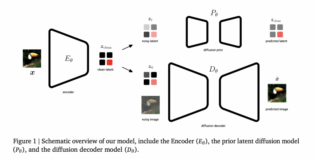
Google DeepMind Introduces Unified Latents (UL): A Machine Learning Framework that Jointly Regularizes Latents Using a Diffusion Prior and Decoder

Generative AI’s current trajectory relies heavily on Latent Diffusion Models (LDMs) to manage the computational cost of high-resolution synthesis. By compressing data into a lower-dimensional latent space, models can scale effectively. However, a fundamental trade-off persists: lower information density makes latents easier to learn but sacrifices reconstruction quality, while higher density enables near-perfect reconstruction but demands greater modeling capacity. Google DeepMind researchers have introduced Unified Latents (UL), a framework designed to navigate this trade-off systematically. The framework jointly regularizes latent representations with a diffusion prior and decodes them via a diffusion model. https://arxiv.org/pdf/2602.17270 The Architecture: Three Pillars of Unified Latents The Unified Latents (UL) framework rests on three specific technical components: Fixed Gaussian Noise Encoding: Unlike standard Variational Autoencoders (VAEs) that learn an encoder distribution, UL uses a deterministic encoder E𝝷 that predicts a single latent zclean. This latent is then forward-noised to a final log signal-to-noise ratio (log-SNR) of λ(0)=5. Prior-Alignment: The prior diffusion model is aligned with this minimum noise level. This alignment allows the Kullback-Leibler (KL) term in the Evidence Lower Bound (ELBO) to reduce to a simple weighted Mean Squared Error (MSE) over noise levels. Reweighted Decoder ELBO: The decoder utilizes a sigmoid-weighted loss, which provides an interpretable bound on the latent bitrate while allowing the model to prioritize different noise levels. The Two-Stage Training Process The UL framework is implemented in two distinct stages to optimize both latent learning and generation quality. Stage 1: Joint Latent Learning In the first stage, the encoder, diffusion prior (P𝝷), and diffusion decoder (D𝝷) are trained jointly. The objective is to learn latents that are simultaneously encoded, regularized, and modeled. The encoder’s output noise is linked directly to the prior’s minimum noise level, providing a tight upper bound on the latent bitrate. Stage 2: Base Model Scaling The research team found that a prior trained solely on an ELBO loss in Stage 1 does not produce optimal samples because it weights low-frequency and high-frequency content equally. Consequently, in Stage 2, the encoder and decoder are frozen. A new ‘base model’ is then trained on the latents using a sigmoid weighting, which significantly improves performance. This stage allows for larger model sizes and batch sizes. Technical Performance and SOTA Benchmarks Unified Latents demonstrate high efficiency in the relationship between training compute (FLOPs) and generation quality. Metric Dataset Result Significance FID ImageNet-512 1.4 Outperforms models trained on Stable Diffusion latents for a given compute budget. FVD Kinetics-600 1.3 Sets a new State-of-the-Art (SOTA) for video generation. PSNR ImageNet-512 Up to 30.1 Maintains high reconstruction fidelity even at higher compression levels. On ImageNet-512, UL outperformed previous approaches, including DiT and EDM2 variants, in terms of training cost versus generation FID. In video tasks using Kinetics-600, a small UL model achieved a 1.7 FVD, while the medium variant reached the SOTA 1.3 FVD. https://arxiv.org/pdf/2602.17270 Key Takeaways Integrated Diffusion Framework: UL is a framework that jointly optimizes an encoder, a diffusion prior, and a diffusion decoder, ensuring that latent representations are simultaneously encoded, regularized, and modeled for high-efficiency generation. Fixed-Noise Information Bound: By using a deterministic encoder that adds a fixed amount of Gaussian noise (specifically at a log-SNR of λ(0)=5) and linking it to the prior’s minimum noise level, the model provides a tight, interpretable upper bound on the latent bitrate. Two-Stage Training Strategy: The process involves an initial joint training stage for the autoencoder and prior, followed by a second stage where the encoder and decoder are frozen and a larger ‘base model’ is trained on the latents to maximize sample quality. State-of-the-Art Performance: The framework established a new state-of-the-art (SOTA) Fréchet Video Distance (FVD) of 1.3 on Kinetics-600 and achieved a competitive Fréchet Inception Distance (FID) of 1.4 on ImageNet-512 while requiring fewer training FLOPs than standard latent diffusion baselines. Check out the Paper. Also, feel free to follow us on Twitter and don’t forget to join our 120k+ ML SubReddit and Subscribe to our Newsletter. Wait! are you on telegram? now you can join us on telegram as well. The post Google DeepMind Introduces Unified Latents (UL): A Machine Learning Framework that Jointly Regularizes Latents Using a Diffusion Prior and Decoder appeared first on MarkTechPost.

Google DeepMind Introduces Unified Latents (UL): A Machine Learning Framework that Jointly Regularizes Latents Using a Diffusion Prior and Decoder Leggi l'articolo »

AI, Committee, Notizie, Uncategorized

Alibaba Team Open-Sources CoPaw: A High-Performance Personal Agent Workstation for Developers to Scale Multi-Channel AI Workflows and Memory

As the industry moves from simple Large Language Model (LLM) inference toward autonomous agentic systems, the challenge for devs have shifted. It is no longer just about the model; it is about the environment in which that model operates. A team of researchers from Alibaba released CoPaw, an open-source framework designed to address this by providing a standardized workstation for deploying and managing personal AI agents. CoPaw is built on a technical stack comprising AgentScope, AgentScope Runtime, and ReMe. It functions as a bridge between high-level agent logic and the practical requirements of a personal assistant, such as persistent memory, multi-channel connectivity, and task scheduling. The Architecture: AgentScope and ReMe Integration CoPaw is not a standalone bot but a workstation that orchestrates multiple components to create a cohesive ‘Agentic App.’ The system relies on three primary layers: AgentScope: The underlying framework that handles agent communication and logic. AgentScope Runtime: The execution environment that ensures stable operation and resource management. ReMe (Memory Management): A specialized module that handles both local and cloud-based memory. This allows agents to maintain ‘Long-Term Experience,’ solving the statelessness issue inherent in standard LLM APIs. By leveraging ReMe, CoPaw allows users to control their data privacy while ensuring the agent retains context across different sessions and platforms. This persistent memory is what enables the workstation to adapt to a user’s specific workflows over time. Extensibility via the Skills System A core feature of the CoPaw workstation is its Skill Extension capability. In this framework, a ‘Skill’ is a discrete unit of functionality—essentially a tool that the agent can invoke to interact with the external world. Adding capabilities to CoPaw does not require modifying the core engine. Instead, CoPaw supports a custom skill directory where engineers can drop Python-based functions. These skills follow a standardized specification (influenced by anthropics/skills), allowing the agent to: Perform web scraping (e.g., summarizing Reddit threads or YouTube videos). Interact with local files and desktop environments. Query personal knowledge bases stored within the workstation. Manage calendars and email via natural language. This design allows for the creation of Agentic Apps—complex workflows where the agent uses a combination of built-in skills and scheduled tasks to achieve a goal autonomously. Multi-Channel Connectivity (All-Domain Access) One of the primary technical hurdles in personal AI is deployment across fragmented communication platforms. CoPaw addresses this through its All-Domain Access layer, which standardizes how agents interact with different messaging protocols. Currently, CoPaw supports integration with: Enterprise Platforms: DingTalk and Lark (Feishu). Social/Developer Platforms: Discord, QQ, and iMessage. This multi-channel support means that a developer can initialize a single CoPaw instance and interact with it from any of these endpoints. The workstation handles the translation of messages between the agent’s logic and the specific channel’s API, maintaining a consistent state and memory regardless of where the interaction occurs. Key Takeaways Shift from Model to Workstation: CoPaw moves the focus away from just the Large Language Model (LLM) and toward a structured Workstation architecture. It acts as a middleware layer that orchestrates the AgentScope framework, AgentScope Runtime, and external communication channels to turn raw LLM capabilities into a functional, persistent assistant. Long-Term Memory via ReMe: Unlike standard stateless LLM interactions, CoPaw integrates the ReMe (Memory Management) module. This allows agents to maintain ‘Long-Term Experience’ by storing user preferences and past task data either locally or in the cloud, enabling a personalized evolution of the agent’s behavior over time. Extensible Python-Based ‘Skills’: The framework uses a decoupled Skill Extension system based on the anthropics/skills specification. Developers can extend an agent’s utility by simply adding Python functions to a custom skill directory, allowing the agent to perform specific tasks like web scraping, file manipulation, or API integrations without modifying the core codebase. All-Domain Multi-Channel Access: CoPaw provides a unified interface for cross-platform deployment. A single workstation instance can be connected to enterprise tools (Lark, DingTalk) and social/developer platforms (Discord, QQ, iMessage), allowing the same agent and its memory to be accessed across different environments. Automated Agentic Workflows: By combining Scheduled Tasks with the skills system, CoPaw transitions from reactive chat to proactive automation. Devs can program ‘Agentic Apps’ that perform background operations—such as daily research synthesis or automated repository monitoring—and push results to the user’s preferred communication channel. Check out the Repo here and Website. Also, feel free to follow us on Twitter and don’t forget to join our 120k+ ML SubReddit and Subscribe to our Newsletter. Wait! are you on telegram? now you can join us on telegram as well. The post Alibaba Team Open-Sources CoPaw: A High-Performance Personal Agent Workstation for Developers to Scale Multi-Channel AI Workflows and Memory appeared first on MarkTechPost.

Alibaba Team Open-Sources CoPaw: A High-Performance Personal Agent Workstation for Developers to Scale Multi-Channel AI Workflows and Memory Leggi l'articolo »

We use cookies to improve your experience and performance on our website. You can learn more at Politica sulla privacy and manage your privacy settings by clicking Settings.

Privacy Preferences

You can choose your cookie settings by turning on/off each type of cookie as you wish, except for essential cookies.

Allow All
Manage Consent Preferences
  • Always Active

Save
it_IT