YouZum

Uncategorized

AI, Committee, Notizie, Uncategorized

Zyphra Releases ZUNA1.1: An Apache 2.0 EEG Foundation Model With Variable-Length Inputs From 0.5 To 30 Seconds

This week, Zyphra released ZUNA1.1 under the Apache 2.0 license. The EEG foundation model reconstructs, denoises, and upsamples data across arbitrary channel layouts. It builds on ZUNA1, the Zyphra’s earlier open EEG foundation model. The main change is flexibility, not a jump in raw accuracy. Real EEG recordings are messy. Sessions vary in length, and channels go noisy or drop out mid-session. Montages range from four-electrode headbands to 256-channel research caps. ZUNA1 processed only fixed five-second segments. ZUNA1.1 accepts variable-length inputs from 0.5 to 30 seconds. What is ZUNA1.1? To understand that flexibility, start with what the model does. ZUNA1.1 is a 380M-parameter masked diffusion autoencoder for scalp-EEG signals. Given a subset of channels, it denoises existing EEG segments and channels. It reconstructs missing ones. It also predicts novel channel signals given physical coordinates on the scalp. The parameter count is unchanged from ZUNA1. It runs on a consumer GPU and works acceptably on CPU for many workloads. Weights sit on Hugging Face; inference and preprocessing code sit on GitHub. Install with pip install zuna. Zyphra also hosts a free browser EEG Playground, and ships all of this for research use only. How The Architecture Works That flexibility rests on tokenization. ZUNA is a transformer encoder–decoder diffusion autoencoder. It slices each channel into 0.125 second segments, which is 32 samples at 256 Hz. Each segment becomes a continuous-valued token. Tokens are serialized in channel × time order. The positional encoding is the key idea. Each token carries a 4D rotary positional encoding over (x, y, z, t). That is the electrode’s 3D scalp coordinate along with its coarse-time index. Because position, not array index, tells the model where a channel sits, ZUNA is channel-agnostic. It accepts any electrode layout, and can generate signals at positions never recorded. That capability enables arbitrary channel upsampling by location. The encoder compresses the signal into a latent. That latent conditions the decoder via adaptive-RMS norm. The decoder is trained with a rectified-flow objective. ZUNA1.1’s architectural changes targeted training stability, such as added normalization layers. What Changed From ZUNA1 Since the architecture stayed close, the differences come from training. 1. Variable-length inputs (0.5–30 seconds): ZUNA1.1 samples a segment length per training example, snapped to the 0.125 s token grid. Lengths are drawn across four bins, from very short to long. The middle 1.5–10 s range is oversampled, since it is the most common operating point. Because token counts vary, Zyphra packs multiple segments per batch up to a fixed budget. Flex attention with a sample-aware mask stops tokens attending across samples. One model therefore serves a 0.5 s snippet and a 30 s stretch without reconfiguration. 2. A richer mixture of reconstruction tasks: ZUNA1 trained on one dropout pattern: uniformly random whole channels. ZUNA1.1 trains on four. The first is whole-channel dropout, covering sparse montages and dead electrodes. The second removes short time stretches across every channel. The third removes those stretches from only some channels, clustering gaps in space and time. The fourth scatters missing values across individual points. 3. Quality-aware preprocessing and a bigger corpus: ZUNA1 made channel-quality calls at the whole-recording level, discarding usable signal. ZUNA1.1 instead computes a per-channel, per-second quality score, thresholded at load time. That grew the corpus from roughly 2M to roughly 3.5M channel-hours of public EEG data. Zyphra team also precomputes two filter variants per recording: a 0.1–45 Hz bandpass, and a 0.01 Hz highpass along with notch. Generalizing across preprocessing strategies is a stated goal, not a benchmarked result. The Results Consequently, the question is whether flexibility cost accuracy. On held-out tasks, ZUNA1.1 reaches better or essentially the same reconstruction NMSE as ZUNA1. Both clearly outperform classical spherical-spline interpolation from MNE. For fair comparison, those evaluation sets used exactly five-second samples. Zyphra also ran a region-based test. Electrodes from one brain region are deleted, then reconstructed from the remaining seven. That setup is more realistic than random channel dropping. ZUNA1.1 outperforms both spherical-spline and ZUNA1 there. Interactive Explainer To make those mechanics concrete, the demo below animates the pipeline end to end. ZUNA1 vs ZUNA1.1 Taken together, the releases differ mostly in training, not architecture. Attribute ZUNA1 ZUNA1.1 Parameters 380M 380M Architecture Transformer encoder–decoder diffusion autoencoder Same, plus extra normalization layers Input length Fixed 5 s 0.5–30 s, snapped to 0.125 s grid Token 0.125 s / 32 samples at 256 Hz Same Positional encoding 4D RoPE over (x, y, z, t) Same Decoder objective Rectified flow Rectified flow Dropout schemes in training 1 (uniform random whole-channel) 4 (channel, time, channel×time, scattered) Training corpus ~2M channel-hours ~3.5M channel-hours Quality filtering Whole-recording level Per-channel, per-second score at load time Preprocessing variants Single Two (0.1–45 Hz bandpass; 0.01 Hz highpass + notch) License Apache 2.0 Apache 2.0 Reconstruction NMSE Baseline Equal or better Running It Turning to practice, reconstruct_fif runs directly on .fif files with no .pt round-trip. The older four-step pipeline still ships alongside it. Copy CodeCopiedUse a different Browser from zuna import reconstruct_fif reconstruct_fif( input_dir=”fif_in”, output_dir=”fif_out”, figures_dir=”figures”, gpu_device=0, # GPU id, or “” for CPU segment_sec=5.0, # window length; default is 5.0, not the full 30 s montage=”standard_1020″, # fallback, used only if the file has no positions repair_channels=[“Cz”], # channel(s) to fully reconstruct target_channel_count=[“Fz”, “Pz”], # add/upsample new channels by name (or an int for auto) bad_segments=[(5, 6), (10, 11, “C3”)], # mark time spans bad (all channels, or one) sample_steps=50, # diffusion steps; note: not “diffusion_sample_steps” ) Note the defaults. segment_sec is 5.0, so the 0.5–30 s range needs setting explicitly. Electrode positions are read from the file itself. The montage argument is only a fallback when positions are absent, and channels without 3D coordinates are dropped. The reconstruction target is a union. It combines the file’s own MNE bad channels and BAD_ annotations with anything requested above. Two directories are written. full_reconstruction/ holds model output everywhere. hybrid/ keeps the original and infills only inferred cells, plus a _mask.npz. Use Cases With Examples Because masking is now flexible, several practical patterns open up.
Zyphra Releases ZUNA1.1: An Apache 2.0 EEG Foundation Model With Variable-Length Inputs From 0.5 To 30 Seconds Leggi l'articolo »

AI, Committee, Notizie, Uncategorized

Sakana AI’s Error Diffusion Trains Dale-Compliant Dual-Stream Networks, Reaching 96.7% MNIST and 61.7% CIFAR-10 Without Backpropagation

Backpropagation dominates deep learning, yet it uses a mechanism the brain likely cannot. Specifically, the backward pass needs exact transposes of forward weight matrices. This is the weight transport problem. Sakana AI’s new paper, Diffusing Blame, confronts this constraint directly. The research team trains networks that obey Dale’s principle while avoiding weight transport entirely. What is Error Diffusion? Error Diffusion (ED) is a local learning rule, first proposed by Kaneko (2000). Each weight update depends on three signals only. These are presynaptic activity, a postsynaptic activation derivative, and a single global error sign. Consequently, ED never transports transposed forward weights or uses random feedback matrices. That locality makes ED naturally compatible with Dale’s principle. However, prior work demonstrated ED only on binary classification and MNIST. The Dual-Stream Architecture To satisfy that constraint, the research team split each layer into two streams. One stream is excitatory (p), and the other is inhibitory (n). The forward pass computes excitatory-minus-inhibitory preactivations for each stream: Copy CodeCopiedUse a different Browser p_i = φ_i( +p_{i-1} Wpp − n_{i-1} Wnp + bp ) n_i = φ_i( +n_{i-1} Wnn − p_{i-1} Wpn + bn ) Here, all four weight matrices stay non-negative element-wise. The biases bp and bn are the exception, since they need not be non-negative. Moreover, the negation signs before Wnp and Wpn are structural, not learned. Therefore cross-stream connections remain inhibitory while all learnable weights stay non-negative. This design needs four weight sub-matrices per layer. As a result, it uses roughly 4× more parameters than a single-stream network. For the same architecture, that is ∼32M versus ∼8M for DFA. Modulo Error Routing With that architecture in place, the main extension is modulo error routing. This lifts Error Diffusion (ED) beyond binary classification. For hidden unit i, the research team define the routing r(i) = i mod C. Here, C is the output dimension. That unit then learns from the routed error component. In short, each hidden unit is assigned one fixed output channel. Unlike DFA, whose feedback matrices are random, ED uses this structured correspondence. Three Classification Innovations Building on that routing, the research team adds three fixes for multi-class classification: Layer-specific sigmoid widths use φi(z) = 1/(1 + e−2z/αi). Since the sigmoid derivative directly gates the error signal, attenuation is severe. In fact, post-hoc analysis reveals a 25× decay from the output to the first hidden layer. Wider sigmoids keep derivatives larger, preventing premature saturation. The team sets α = 3.0 for CIFAR-10 convolutional layers and α = 6.0 for fully connected layers. Batch-centered class error subtracts the per-class mini-batch mean. This makes the one-vs-all error zero-mean across the batch for every class. It thereby reduces persistent suppression caused by the 9:1 target imbalance. Asymmetric initialization scales excitatory weights by 1.5× and inhibitory weights by 0.5×. That gives an expected E/I scale ratio of 3:1, while the output layer stays symmetric. Performance With all three innovations, Error Diffusion (ED) reaches 96.7% on MNIST and 61.7% on CIFAR-10. In contrast, seed ED without them collapses to 50.4% and 11.6%. DFA scores higher on both tasks but violates Dale’s principle, using ∼2.84M negative weights. Notably, this is the first time ED has trained convolutional networks. Previously, Fujita (2026) reached ∼55.2% on CIFAR-10 using a flattened MLP. Even so, 61.7% remains far from standard gradient-based methods. Method MNIST CIFAR-10 Dale-compliant Notes Proposed ED 96.7% 61.7% Yes All weights non-negative; first ED on CNNs Seed ED 50.4% 11.6% Yes No innovations; α = 1.0, raw error, symmetric init DFA 97.6% 69.1% No Random feedback; ∼2.84M negative weights The Ablation Reversal Interestingly, the innovations’ importance flips between tasks. On MNIST, removing layer-specific widths is catastrophic (−71.4 pp), collapsing accuracy toward chance. Batch-centering barely matters there (−0.3 pp). On CIFAR-10, however, the order reverses. Removing batch-centered error becomes the largest drop (−47.9 pp), collapsing four of five seeds. This reversal exposes task-dependent credit-assignment bottlenecks invisible to single-benchmark evaluation. Error Diffusion in Reinforcement Learning Beyond classification, the research team integrate ED with Proximal Policy Optimization (PPO). They call the result ED-PPO and test it on Brax locomotion and Craftax. Here, policy-output error is routed to hidden units by output channel. For the scalar value network, the error is broadcast to all units. Importantly, ED-PPO drops the three classification innovations entirely. Across five seeds, ED-PPO beats BP-PPO on HalfCheetah (5494 vs 3520; p < 0.001) and matches DFA-PPO. On Ant, it stays on par with both PPO variants. On Craftax, meanwhile, DFA-PPO is the weakest method (19.8 vs BP-PPO 27.0). Thus random feedback that suffices for classification can fail on open-ended RL. Use Cases and Examples Three settings make this concrete: Neuromorphic and photonic hardware often encodes non-negative synaptic magnitudes physically. ED’s fixed-sign routing maps cleanly onto such substrates, complementing prior photonic DFA work. The non-negative floor drives 37.3% of weights to the floor (10⁻⁴) after training. Inhibitory cross-stream fully connected connections are pruned most, up to 68.8%. This implicit sparsity hints at model compression “for free.” The dedicated inhibitory stream may help continual and open-ended learning. It provides a structural mechanism for dampening large gradient excursions. Comparison How Dale-Compliant Error Diffusion Compares Proposed approach vs. other backpropagation-free and biologically motivated learning rules. “Dale-compliant” means separate excitatory/inhibitory populations with non-negative weights. Method names link to primary sources. Method Backprop-free (no weight transport) How error reaches hidden layers Dale-compliant (E/I, non-negative) Shown on RL Demonstrated reach / notes Error Diffusion — ED / ED-PPO (proposed) Yes Global error sign routed directly to hidden units via modulo routing r(i) = i mod C Yes — dual-stream E/I, non-negative weights Yes (Brax, Craftax) 96.7% MNIST, 61.7% CIFAR-10; RL returns on par with DFA-PPO Backpropagation No — needs transposed forward weights Exact gradient, layer by layer No — arbitrary-sign weights Yes (BP-PPO) Reference baseline; state of the art across tasks Feedback Alignment (FA) Yes Fixed random backward weights, layer by layer No — arbitrary-sign feedback Not shown Learns deep and convolutional nets; limited on harder benchmarks Direct Feedback Alignment (DFA) Yes Output error to

Sakana AI’s Error Diffusion Trains Dale-Compliant Dual-Stream Networks, Reaching 96.7% MNIST and 61.7% CIFAR-10 Without Backpropagation Leggi l'articolo »

AI, Committee, Notizie, Uncategorized

Build an Agentic Event Venue Operator with MongoDB Atlas, Voyage, and LangGraph

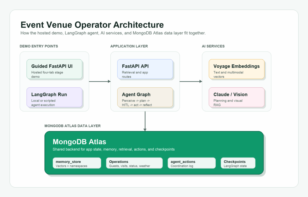
Introduction This tutorial starts where most agent demos stop: giving the agent persistent memory, operational context, and a place to write back what happened. An event operator does not just need an agent that can summarize a weather report or generate a generic plan. The operator needs an agent that can remember what happened at prior events, retrieve relevant visitor and venue context, respond to live operational changes, and write the outcome back as memory for the next similar situation. We built this event-venue operator demo with MongoDB Atlas, Voyage AI embeddings, LangGraph, and optional Langfuse tracing. The demo scenario is the MongoDB Open, a fictional premium tennis tournament on Day 6 of play. Rain is approaching, covered hospitality capacity is constrained, and the operator has two different visitor journeys to protect: Mikiko, a first-time attendee trying to make the most of the grounds, and Nina, a premier guest with hospitality expectations and a history the agent can retrieve. This is not a customer case study or a production deployment. It is a fictional builder scenario inspired by real event operations economics. Major tennis events show why these decisions matter: the 2025 US Open broke attendance, viewership, and digital reach records and offered $90 million in total player compensation; USTA has also said the three-week US Open drives more than $1.2 billion in annual economic impact for New York City. Premium fan expectations are high, too: PwC found that 60% of high-income U.S. sports fans would spend more than $250 for a special event, and 20% would spend more than $1,000. Weather adds another layer of risk, which is why the U.S. Census Bureau now tracks the monetary impact of extreme weather on business sales through its Business Trends and Outlook Survey. The MongoDB Open demo agent is not just producing a plausible plan. It reads current venue state, retrieves prior event memory, distinguishes between visitor segments, and acts. At the same time, hospitality capacity is still available, and writes the outcome back so the next disruption can be handled with more context. Check out the full repo here.  The demo is split into three layers: A guided, deterministic UI that makes the operator story easy to follow. A hosted Vercel demo that gives readers a public app link. Live API endpoints and scripts for Atlas Vector Search, vector-plus-lexical retrieval, visual-document RAG, LangGraph execution, and optional Langfuse traces, to demonstrate how the stack all works together.  What You Will Build By the end of the tutorial, you will have a FastAPI app backed by MongoDB Atlas that can run locally and deploy to Vercel. The app includes: A four-tab guided UI for the event-operations story and live backend validation. Atlas collections for operational state, semantic memory, agent actions, and LangGraph checkpoints. Voyage multimodal embeddings stored in Atlas. Atlas Vector Search for memory retrieval. A hybrid retrieval endpoint that combines vector similarity with lexical scoring. A Vision RAG endpoint that retrieves visual operational documents and passes them to Claude Vision. Optional Langfuse tracing for retrieval calls and the live LangGraph run. A runnable LangGraph script that follows the same rain-delay story. A Vercel deployment configuration for a hosted demo. The current repo should be treated as a reference demo, not a production platform. There is no production auth, no CI suite, and the full LangGraph agent remains a script-based validation path rather than a public hosted endpoint. Architecture Overview The architecture centers on MongoDB Atlas as both the operational and memory layer. Speed matters in the event venue operator scenario because the useful window for action is short. If rain is 20 minutes away and covered hospitality space is filling up, the operator does not need a post-event dashboard or a batch summary a few minutes later. The agent needs to read the current venue state, retrieve relevant memory, decide what to do, and write back the result while there is still capacity to protect the guest experience. That is why the type of database and how it is used are critical system design choices. Operational records, semantic memory, vector embeddings, visual documents, and agent actions all live in the same data layer. The agent does not need to wait for a separate analytics pipeline, sync data into a second vector database, or reconcile what the memory layer says with what the operational system says. Atlas acts as both the system of record and the retrieval layer for the agent loop: perceive what changed, retrieve the right context, take action, and persist what happened for the next event. This is also why the demo keeps memory in MongoDB rather than treating it as a sidecar. The agent is not just retrieving chunks; it is composing operational context. A useful decision may need visitor history, current venue status, hospitality inventory, prior rain-delay patterns, and relevant visual documents at the same time. With Atlas, those pieces can stay queryable together instead of being scattered across separate systems. Caption: MongoDB Atlas stores the demo’s operational state, semantic memory, visual document embeddings, agent actions, and LangGraph checkpoints in one backend. The demo uses four main state layers: Operational records: guests, visits, venue status, weather events, reservations, event metrics, and agent actions. Semantic memory: memory_store, with Voyage embeddings and Atlas Vector Search. Visual documents: operational images embedded into the same memory store as image-derived multimodal embeddings and document metadata. Agent state: LangGraph checkpoints and checkpoint writes. Setup Before you begin, make sure you have: Python 3.12 or later uv installed A MongoDB Atlas cluster with Vector Search enabled (this can be set up for free) An Anthropic API key (or feel free to use an LLM of your choice and reconfigure API keys) A Voyage API key (this can be set up for free) Clone the repo and install dependencies: GitHub repo Copy CodeCopiedUse a different Browser git clone https://github.com/mongodb-developer/event-venue-operator.git cd event-venue-operator uv sync If you only want to inspect the app before setting up credentials, start with the live Vercel demo. The hosted demo

Build an Agentic Event Venue Operator with MongoDB Atlas, Voyage, and LangGraph Leggi l'articolo »

AI, Committee, Notizie, Uncategorized

Google Cloud’s Always-On Memory Agent Replaces RAG and Embeddings With Continuous LLM Consolidation on Gemini 3.1 Flash-Lite

Most AI agents forget. They process a request, answer it, then drop the context. Google Cloud’s generative-ai repository now ships a sample that tackles this directly. It is the Always-On Memory Agent, a reference implementation that treats memory as a running process. Always-On Memory Agent Fundamentally, the project is a lightweight background agent that never stops. It runs 24/7 as a continuous process, not a one-shot call. It is built with Google ADK (Agent Development Kit) and Gemini 3.1 Flash-Lite. Notably, it uses no vector database and no embeddings. Instead, an LLM reads, thinks, and writes structured memory into SQLite. The model choice targets low latency and low cost for continuous background work. How It Works: Ingest, Consolidate, Query Architecturally, an orchestrator routes every request to one of three specialist sub-agents. Each sub-agent owns its own tools for reading or writing the memory store. First, the IngestAgent handles incoming content. It uses Gemini’s multimodal capabilities to extract a summary, entities, topics, and an importance score. That structured record then lands in the memories table. Next, the ConsolidateAgent runs on a timer, every 30 minutes by default. Like sleep cycles, it reviews unconsolidated memories and finds connections between them. Then it writes a synthesized summary, one key insight, and those connections to the database. Consequently, the agent builds new understanding while idle, with no prompt. Finally, the QueryAgent answers questions. It reads all memories and consolidation insights, then synthesizes a response. Importantly, it cites the memory IDs it used as sources. “, src:”report.pdf”, sm:”Anthropic reports 62% of Claude usage is code-related.”, ent:[“Anthropic”,”Claude”,”AI agents”], tp:[“AI”,”code generation”], imp:0.8}, {icon:”“, src:”roadmap.png”, sm:”Q1 priority: reduce inference costs by 40%.”, ent:[“Q1″,”inference”], tp:[“cost”,”planning”], imp:0.7}, {icon:”“, src:”standup.mp3″, sm:”AI agents grow fast, but reliability is still a challenge.”, ent:[“AI agents”,”reliability”], tp:[“agents”,”reliability”], imp:0.75}, {icon:”“, src:”idea.txt”, sm:”Smart inbox idea: persistent AI memory for email.”, ent:[“smart inbox”,”email”], tp:[“product”,”memory”], imp:0.6} ]; var CONS = { links:[[1,3],[2,1],[3,4]], insight:”The bottleneck for next-gen AI tools is the transition from static RAG to dynamic memory systems.” }; var Q = “What should I focus on?”; var A = ‘Based on your memories, prioritize: ship the cost-reduction plan <span class="”ref”">[Memory 2]</span>, ‘ + ‘then close the agent reliability gap <span class="”ref”">[Memory 3]</span>. ‘ + ‘The smart inbox concept <span class="”ref”">[Memory 4]</span> validates demand for persistent AI memory.’; var i=0, consolidated=false; var $=function(id){return document.getElementById(id)}; var store=$(“store”), pkt=$(“pkt”), logEl=$(“log”); function post(){ try{ parent.postMessage({type:”aoma-resize”,height:document.body.offsetHeight+40},”*”); }catch(e){} } function log(html){ logEl.innerHTML=html; post(); } function activate(el,cls){ [ “sIngest”,”sCons”,”sQuery” ].forEach(function(id){ $(id).classList.remove(“active”,”cons”,”query”); }); if(el){ el.classList.add(“active”); if(cls) el.classList.add(cls); } } function packet(color){ pkt.style.background=color; pkt.style.opacity=”1″; pkt.style.left=”0″; setTimeout(function(){ pkt.style.left=”calc(100% – 10px)”; },30); setTimeout(function(){ pkt.style.opacity=”0″; },950); } function ingest(){ if(i>=SAMPLES.length){ log(“<b>Inbox empty.</b> All 4 sample files ingested — now consolidate or query.”); return; } var s=SAMPLES[i]; var id=i+1; activate($(“sIngest”)); packet(“#4285F4”); log(‘<b>IngestAgent</b> reads <b>’+s.icon+’ ‘+s.src+'</b> → extracting summary, entities, topics, importance…’); var c=document.createElement(“div”); c.className=”card”; c.id=”card”+id; c.innerHTML='<span class="”cid”">#’+id+'</span><div class="”sm”">’+s.sm+'</div>’+ ‘<div class="”chips”">’+s.ent.map(function(e){return ‘<span class="”chip”">’+e+'</span>’}).join(“”)+'</div>’+ ‘<div class="”chips”">’+s.tp.map(function(t){return ‘<span class="”chip" tp”>’+t+'</span>’}).join(“”)+'</div>’+ ‘<div class="”imp”">importance <b>’+s.imp+'</b></div>’; store.appendChild(c); post(); setTimeout(function(){ c.classList.add(“show”); post(); log(‘<b>Stored memory #’+id+'</b> in SQLite. ‘+(SAMPLES.length-id)+’ file(s) left in inbox.’); },500); i++; if(i>=2){ $(“bCons”).disabled=false; $(“bQuery”).disabled=false; } } function consolidate(){ if(i<2){ log(“Ingest at least 2 memories first.”); return; } activate($(“sCons”),”cons”); packet(“#FBBC04”); $(“tmr”).classList.add(“run”); log(“<b>ConsolidateAgent</b> woke on its 30-min timer — reviewing unconsolidated memories…”); var svg=$(“wires”); svg.innerHTML=””; for(var k=1;k<=Math.min(i,4);k++){ var el=$(“card”+k); if(el) el.classList.add(“hl”); } setTimeout(function(){ CONS.links.forEach(function(pair){ drawWire(pair[0],pair[1]); }); log(“<b>Found connections</b> across memories — writing one cross-cutting insight…”); },500); setTimeout(function(){ var ins=$(“insight”); ins.innerHTML='<b>Insight:</b> ‘+CONS.insight; ins.classList.add(“show”); $(“tmr”).classList.remove(“run”); consolidated=true; log(“<b>Consolidation done.</b> New insight written back to the store — no prompt needed.”); post(); },1200); } function drawWire(a,b){ var svg=$(“wires”), ca=$(“card”+a), cb=$(“card”+b); if(!ca||!cb) return; var box=svg.getBoundingClientRect(), ra=ca.getBoundingClientRect(), rb=cb.getBoundingClientRect(); var x1=ra.left-box.left+ra.width/2, y1=ra.top-box.top+ra.height/2; var x2=rb.left-box.left+rb.width/2, y2=rb.top-box.top+rb.height/2; var ln=document.createElementNS(“http://www.w3.org/2000/svg”,”line”); ln.setAttribute(“x1”,x1);ln.setAttribute(“y1”,y1);ln.setAttribute(“x2”,x1);ln.setAttribute(“y2”,y1); ln.setAttribute(“stroke”,”#FBBC04″);ln.setAttribute(“stroke-width”,”2″);ln.setAttribute(“stroke-dasharray”,”4 3″); svg.appendChild(ln); requestAnimationFrame(function(){ ln.style.transition=”all .5s”; ln.setAttribute(“x2”,x2); ln.setAttribute(“y2”,y2); }); } function query(){ if(i<1){ log(“Ingest something first.”); return; } activate($(“sQuery”),”query”); packet(“#34A853”); $(“qbox”).classList.add(“show”); $(“qask”).textContent=’Q: ‘+Q; $(“qans”).innerHTML=”Reading all memories…”; log(“<b>QueryAgent</b> reads every memory”+(consolidated?” and the consolidation insight”:””)+”, then synthesizes…”); [“card2″,”card3″,”card4”].forEach(function(id){ var el=$(id); if(el) el.classList.add(“cite”); }); setTimeout(function(){ $(“qans”).innerHTML=A; log(“<b>Answer returned</b> with cited memory IDs — grounded only in stored memories.”); post(); },900); } function reset(){ i=0; consolidated=false; store.innerHTML=””; $(“wires”).innerHTML=””; $(“insight”).className=”insight”; $(“insight”).innerHTML=””; $(“qbox”).className=”qbox”; $(“qans”).innerHTML=””; $(“qask”).textContent=””; $(“bCons”).disabled=true; $(“bQuery”).disabled=true; activate(null); log(“<b>Reset.</b> Drop a file into the agent’s inbox to begin.”); } $(“bIngest”).onclick=ingest; $(“bCons”).onclick=consolidate; $(“bQuery”).onclick=query; $(“bReset”).onclick=reset; window.addEventListener(“load”,post); window.addEventListener(“resize”,post); if(window.ResizeObserver){ new ResizeObserver(post).observe(document.body); } setTimeout(post,150); })(); </script> </body> </html> “> Supported Inputs Beyond text, the IngestAgent accepts 27 file types across five categories. Simply drop any supported file into the ./inbox folder for automatic pickup. Category Extensions Text .txt, .md, .json, .csv, .log, .xml, .yaml, .yml Images .png, .jpg, .jpeg, .gif, .webp, .bmp, .svg Audio .mp3, .wav, .ogg, .flac, .m4a, .aac Video .mp4, .webm, .mov, .avi, .mkv Documents .pdf How It Compares to RAG, Summaries, and Knowledge Graphs To clarify the difference, it frames three common memory approaches. Each solves part of the problem, yet leaves a gap. Approach How it stores Active processing Main limitation Vector DB + RAG Embeddings in a vector store None Passive; embeds once, retrieves later Conversation summary Compressed text None Loses detail; no cross-reference Knowledge graphs Nodes and edges Manual upkeep Expensive to build and maintain Always-On Memory Agent Structured rows in SQLite Continuous consolidation Query reads up to 50 recent memories Unlike RAG, this agent processes memory actively, not only on retrieval. Use Cases With Examples Practically, the pattern fits any workload needing durable, evolving context. Consider three examples. A research assistant ingests PDFs, meeting audio, and screenshots all week. Later, it links a cost target to a reliability problem on its own. A personal knowledge base absorbs notes, articles, and images continuously. Over time, consolidation surfaces themes you never explicitly connected. A support agent stores past tickets as structured memories. Then it answers new questions with cited references to earlier cases. Getting Started With the design clear, setup stays minimal for early-level engineers. Install dependencies, set your key, then start the process. Copy CodeCopiedUse a different Browser pip install -r requirements.txt export GOOGLE_API_KEY=”your-gemini-api-key” python agent.py Once running, the agent watches ./inbox, consolidates every 30 minutes, and serves an HTTP API on port 8888. Therefore, you can also feed it over HTTP. Copy CodeCopiedUse a different Browser #

Google Cloud’s Always-On Memory Agent Replaces RAG and Embeddings With Continuous LLM Consolidation on Gemini 3.1 Flash-Lite Leggi l'articolo »

AI, Committee, Notizie, Uncategorized

NVIDIA Released DeepStream 9.1: Bringing Agentic AI to Vision AI With 13 Skills and Multi-View 3D Tracking

NVIDIA just released DeepStream 9.1. The update targets a persistent problem in video analytics. Tracking one object across many cameras traditionally requires manual camera calibration and complicated calculations. DeepStream 9.1 addresses this with two additions: Multi-View 3D Tracking (MV3DT) and AutoMagicCalib (AMC). Both ship as agentic skills for coding agents. As a result, developers move from concept to a running pipeline faster. What is DeepStream 9.1 To understand the update, start with the base platform. DeepStream is NVIDIA’s streaming analytics toolkit for AI-based video and image understanding. It provides a GStreamer-based framework for multi-stream, multi-model inference on NVIDIA GPUs. Pipelines combine hardware-accelerated decoding and encoding, TensorRT inference, object tracking, and message-broker integration. Building on that base, version 9.1 adds five notable items: 13 agentic skills for coding agents. The MV3DT skill for cross-camera tracking. The AMC skill for automatic calibration. NVIDIA JetPack 7.2 support for Jetson Orin and Thor edge devices. A unified open-source GitHub repository under CC-BY-4.0 AND Apache-2.0. How MV3DT Tracks Objects Across Cameras Among those additions, MV3DT is the main skill, so consider how it works. At its core, MV3DT projects detections from multiple calibrated cameras into a shared 3D coordinate system. It then associates observations of the same object across camera views. Finally, it assigns one globally consistent object ID. Concretely, the data flow runs in four stages. For detection, each camera stream runs an object detector. MV3DT supports three models out of the box: PeopleNetTransformer: a transformer-based people detector, the default for pedestrian scenes. PeopleNet v2.6.3: a high-efficiency detector based on the DetectNet_v2 architecture. RT-DETR 2D: a multi-class detector for pedestrians, transporters, and forklifts. Next, for monocular 3D perception, each camera uses a 3×4 projection matrix stored in a YAML calibration file. This back-projects 2D bounding boxes into 3D world-space coordinates using a ground-plane assumption. Then, for multi-view association, the tracker shares tracklets using Message Queuing Telemetry Transport (MQTT). MQTT is a lightweight pub/sub messaging protocol. When two cameras observe the same person, it matches tracklets by proximity in 3D world space. After association, results stream out in three forms. The On-Screen Display (OSD) shows a tiled grid with 2D and 3D bounding boxes. The Bird’s-Eye View (BEV) renders a top-down trajectory map. Kafka messaging delivers per-frame protobuf metadata, including sensor ID, object ID, and 3D bounding box. How AutoMagicCalib Removes Manual Setup MV3DT depends on calibrated cameras, which traditionally means checkerboards and downtime. Instead, AMC calibrates a network by analyzing tracked objects in existing video files or streams. It estimates each camera’s intrinsic parameters (focal length, principal point, lens distortion). It also estimates extrinsic parameters (rotation, translation, world position). Under the hood, the pipeline runs five stages. These are per-camera trajectory extraction, single-view rectification, multi-view tracklet matching, bundle adjustment, and optional VGGT refinement. VGGT (Visual Geometry Grounded Transformer) helps when object movement is limited. AMC runs as a microservice with REST APIs and a web interface. Users supply only a layout image and a few alignment points. The Agentic Skills Workflow With MV3DT and AMC defined, the delivery mechanism is the skills themselves. Rather than editing configuration files, you describe intent in natural language. The skills work with Claude Code, Codex, Cursor, and similar agents. Setup is short: Copy CodeCopiedUse a different Browser git clone https://github.com/NVIDIA/DeepStream.git cd DeepStream # Copy skills into your agent’s skill directory (Codex shown) mkdir -p ~/.codex/skills cp -r skills/* ~/.codex/skills/ After launching the agent, a single prompt runs the reference app: Copy CodeCopiedUse a different Browser deploy mv3dt on the 12-camera sample dataset From there, the MV3DT skill validates prerequisites, pulls the container, and installs Kafka and Mosquitto broker services. It also downloads model weights, generates the pipeline config, and launches tracking. Notably, if calibration files are missing, it triggers the AMC skills automatically. DeepStream 9.0 vs 9.1 For context, the table below shows what changed between releases. Capability DeepStream 9.0 DeepStream 9.1 Agentic skills 2 (deepstream-dev, import-vision-model) 13 agentic skills Multi-camera 3D tracking Not shipped as a skill MV3DT skill + reference app Camera calibration Manual AutoMagicCalib (AMC) microservice Jetson support JetPack 7.1 GA JetPack 7.2 (Orin, Thor) Sample datasets — 4-camera and 12-camera MV3DT sets Distribution NGC packages + GitHub source Unified GitHub monorepo Use Cases With Examples Given these capabilities, the features map to concrete deployments: Warehouse safety: track a worker near forklifts across aisles with one ID, using RT-DETR 2D. Retail analytics: follow a shopper between camera zones to measure dwell time without re-identification errors. Smart-building monitoring: count occupancy across floors and feed Kafka metadata to dashboards. Robotics and smart cities: share consistent world coordinates for navigation and incident review. Interactive Explainer To see the mechanism, the embedded demo below animates one person walking between three camera fields of view. Toggle between naive per-camera 2D tracking and MV3DT 3D fusion to watch the object ID stay consistent. Key Takeaways DeepStream 9.1 ships 13 agentic skills, letting coding agents build multi-camera vision pipelines from natural-language prompts. MV3DT fuses per-camera detections into one shared 3D world, keeping a single globally consistent object ID across views. AutoMagicCalib replaces manual checkerboard calibration by estimating camera intrinsics and extrinsics from existing video. JetPack 7.2 support extends deployment to Jetson Orin and Thor, under a unified open-source GitHub monorepo. Outputs stream as OSD, Bird’s-Eye View, and Kafka protobuf metadata, ready for downstream analytics and dashboards. Check out the Repo here. Also, feel free to follow us on Twitter and don’t forget to join our 150k+ML SubReddit and Subscribe to our Newsletter. Wait! are you on telegram? now you can join us on telegram as well. Need to partner with us for promoting your GitHub Repo OR Hugging Face Page OR Product Release OR Webinar etc.? Connect with us The post NVIDIA Released DeepStream 9.1: Bringing Agentic AI to Vision AI With 13 Skills and Multi-View 3D Tracking appeared first on MarkTechPost.

NVIDIA Released DeepStream 9.1: Bringing Agentic AI to Vision AI With 13 Skills and Multi-View 3D Tracking Leggi l'articolo »

AI, Committee, Notizie, Uncategorized

NVIDIA AI Releases Nemotron 3 Embed: An Open Embedding Collection Whose 8B Checkpoint Ranks #1 on RTEB

Embedding models decide which passages an agent ever sees. NVIDIA released Nemotron 3 Embed model to work on that layer. It targets production-scale RAG, agentic retrieval, code retrieval, and agent memory. What is Nemotron 3 Embed? The model collection includes three open checkpoints. Nemotron-3-Embed-8B-BF16 is the accuracy-first option. Nemotron-3-Embed-1B-BF16 carries the same design into a smaller footprint. Nemotron-3-Embed-1B-NVFP4 is the Blackwell-optimized 4-bit path. All three are transformer encoders trained with bidirectional attention masking. The final embedding comes from average pooling over token-level representations. Maximum sequence length is 32,768 tokens on every checkpoint. Each model was evaluated across 34 languages. All three carry the OpenMDW License Agreement, version 1.1 (OpenMDW-1.1). Notably, the bases are Mistral models. The 8B is built with Ministral-3-8B-Instruct-2512. Both 1B variants use Ministral-3-3B-Instruct-2512. Performance Nemotron-3-Embed-8B-BF16 ranks #1 overall on RTEB (as of July 17 2026), the Retrieval Embedding Benchmark. Evaluation covers its 16 public tasks. Every figure below is average NDCG@10, at model sequence length 4096. Model Params Emb dim RTEB ViDoRe-V3 text MMTEB (Retrieval) Nemotron-3-Embed-8B-BF16 ~8B 4096 78.46 60.60 75.45 Nemotron-3-Embed-1B-BF16 1.14B 2048 72.38 57.74 71.04 Nemotron-3-Embed-1B-NVFP4 1.14B 2048 72.00 — — llama-nemotron-embed-vl-1b-v2 — — 61.98 52.54 59.71 llama-nemotron-embed-1b-v2 — — 60.47 52.10 59.58 Two gaps are worth noting. The 1B gains 10.4 RTEB points over llama-nemotron-embed-vl-1b-v2, the prior-generation baseline. Separately, NVFP4 costs 0.38 RTEB points against its BF16 parent, or 99.5% retention. How the 1B Model was Built? Those 1B scores come from a compression pipeline, not a smaller training run. The parent was nemotron-3-embed-3b, pruned and distilled across two iterative rounds. First, the 3B parent was pruned to 2B using NVIDIA ModelOpt mcore_minitron Neural Architecture Search (NAS). The search covers hidden width, FFN size, attention heads, and depth. It then picks the best candidate from the top-10 Pareto front. A 50k in-domain calibration corpus scored those candidates. Next, the 2B model was distilled from the fine-tuned 8B embedding teacher. Distillation combined cosine distance loss (COS) and mean squared error (MSE) loss. The data blend was multilingual and in-domain. Finally, the same procedure repeated to produce the 1.14B checkpoint. The NVFP4 Serving Tradeoff Compression then continues into the serving format. Quantization hit weights and activations of linear layers only, targeting the NVFP4 data type. The research team used nvidia-modelopt v0.45.0. Quantization-Aware Distillation (QAD) followed, primarily to recover accuracy on long inputs. Calibration used 512 samples: 256 queries and 256 passages from abisee/cnn_dailymail. QAD training used 20k samples. The rsesearch team reports NVFP4 on Blackwell delivers up to 2x higher throughput than BF16. It retains 99%+ of BF16 retrieval accuracy. The NVFP4 card also documents dynamic embedding sizes. You can slice the 2048-d vector from the start to 1024 or 512 dimensions. Re-normalize afterward. Interactive Explainer: The Five-Stage Retrieval Path Before touching code, watch the path run. It animates prefixing, bidirectional encoding, average pooling, L2 normalization, and dot-product scoring. Scores come from each card’s published expected output. Deployment Matrix As that walkthrough implies, the checkpoints do not share runtime paths. Feature 8B-BF16 1B-BF16 1B-NVFP4 Transformers / Sentence Transformers Yes Yes No vLLM for /v2/embed 0.25.0 0.25.0 0.25.0 Microarchitectures Ampere, Hopper, Blackwell Ampere, Hopper, Blackwell Ampere, Hopper, Lovelace, Blackwell Test hardware A100 80GB, H100 80GB A100 80GB, H100 80GB GB200, RTX 6000 PRO, A100, H100, L40, L4 Training data 50M+ samples 8.5M+ (distillation) 20k (QAD) Alongside the checkpoints, NVIDIA research team released an optimized NIM microservice for the 1B model. The Rust-based NIM matches or outperforms the vLLM checkpoint on GB200 and RTX PRO 6000. NVIDIA tested input sequence lengths of 256 and 1024. Separately, NVIDIA NeMo AutoModel recipes cover fine-tuning and distillation. Using It in Code With those paths in mind, prefixes come first. Queries take query: and documents take passage: . Embeddings are L2-normalized, so dot product equals cosine similarity. Copy CodeCopiedUse a different Browser # pip install –upgrade “transformers>=5.2.0” “sentence-transformers>=5.4.1” import torch from sentence_transformers import SentenceTransformer QUERIES = [“How can someone reduce exposure to pollen during allergy season?”] DOCUMENTS = [“People with pollen allergy can reduce exposure by staying indoors ” “on dry, windy days, avoiding early-morning outdoor activity, and ” “going outside after rain when pollen levels are lower.”] model = SentenceTransformer( “nvidia/Nemotron-3-Embed-8B-BF16″, device=”cuda”, model_kwargs={“dtype”: torch.bfloat16, # use “sdpa” if FlashAttention-2 is unavailable “attn_implementation”: “flash_attention_2”}, processor_kwargs={“padding_side”: “left”}, ) model.max_seq_length = 32768 q = model.encode_query(QUERIES, batch_size=1, convert_to_tensor=True) d = model.encode_document(DOCUMENTS, batch_size=1, convert_to_tensor=True) print(model.similarity(q, d)) # card’s published q[3]/d[3] score: 0.8008 encode_query and encode_document read the saved prompts. So you never add prefixes by hand. For serving, /v2/embed applies them from input_type instead: Copy CodeCopiedUse a different Browser vllm serve nvidia/Nemotron-3-Embed-1B-NVFP4 –max-model-len 4096 –max-num-batched-tokens 4096 –max-cudagraph-capture-size 4096 Copy CodeCopiedUse a different Browser import numpy as np, requests def embed(input_type: str, texts: list[str]) -> np.ndarray: r = requests.post( “http://localhost:8000/v2/embed”, json={“model”: “nvidia/Nemotron-3-Embed-1B-NVFP4”, “input_type”: input_type, # “query” or “document” “texts”: texts, “embedding_types”: [“float”], “truncate”: “END”}, timeout=120, ) r.raise_for_status() return np.array(r.json()[“embeddings”][“float”], dtype=np.float32) scores = embed(“query”, QUERIES) @ embed(“document”, DOCUMENTS).T Use Cases With Examples Multilingual enterprise search: A support team indexes Hindi, Japanese, and English tickets together. Because retrieval is cross-lingual, a German query can surface a Japanese resolution note. Code retrieval: Training included coir_apps, coir_cosqa, synthetic_text2sql, and SWE-bench. Natural-language-to-code lookup is therefore closer to in-distribution. Agent memory: The 32,768-token limit lets an agent embed long conversation summaries without aggressive chunking. Cost-tiered RAG: Serve 1B-NVFP4 for high-volume recall, and route hard queries to the 8B. Because widths differ, this needs two indexes. Key Takeaways Nemotron-3-Embed-8B-BF16 ranks #1 on RTEB at 78.46 avg NDCG@10. Three open checkpoints span 8B BF16, 1B BF16, and 1B NVFP4. NVFP4 retains 99%+ of BF16 accuracy at up to 2x Blackwell throughput. The 1B came from ModelOpt NAS pruning plus COS+MSE distillation from the 8B. All checkpoints use OpenMDW-1.1 and support 32,768-token inputs. Check out the NVIDIA launch post on Hugging Face, Nemotron 3 Embed collection, 8B-BF16 card, 1B-BF16 card and 1B-NVFP4 card. Also, feel free to follow us on Twitter and don’t forget to join our 150k+ML SubReddit and Subscribe to our Newsletter. Wait! are you on telegram? now you can join us on telegram as well. Need to partner with us for

NVIDIA AI Releases Nemotron 3 Embed: An Open Embedding Collection Whose 8B Checkpoint Ranks #1 on RTEB Leggi l'articolo »

AI, Committee, Notizie, Uncategorized

There’s a lot of hype around perimenopause. Don’t buy it.

Perimenopause has entered the chat. Perimenopause—and its better-known relative, menopause—used to be considered taboo. Not anymore, thanks at least in part to TV doctors and social media influencers. Perhaps it’s my age, but these days, both my algorithm and my conversations with friends increasingly swing toward perimenopause. Menopause is defined as the life stage that occurs a year after a person has had their last period. Perimenopause is the sometimes years-long period before that point, which can also feature all the symptoms we’d typically associate with menopause. Today, information about perimenopause is more prevalent and accessible than ever. If you’re a woman in your 40s and you’re not feeling 100%, chances are there’ll be someone online ready to tell you you’re in perimenopause. And that you might want to start spending your money on blood tests, apps, and supplements or demanding hormone replacement therapy. But as regular readers might have guessed by this point, it’s not that simple. Perimenopause tends to start around the age of 46 or 47. It’s during this time that many women start to experience some symptoms like hot flashes, irregular or unusually heavy periods, or anxiety, for example. And it can be heavy going. “Often symptoms are at their worst in the perimenopause,” says Mary Ann Lumsden, former president of the International Menopause Society. That’s because hormones can fluctuate wildly. Levels of estrogen, progesterone, luteinizing hormone, and follicle-stimulating hormone can roller-coaster before leveling off after menopause. And that’s why, despite what some marketers will claim, there is no test for perimenopause. “You can’t interpret hormone [measures] because they change so much,” says Lumsden. “And that is quite normal.” That doesn’t mean women should have to put up with symptoms. But exactly how those symptoms are treated is another topic that has been clouded by misinformation. Last week, I told a friend about some unusually bad pelvic pain I’d experienced. Her immediate advice was to find out if I was perimenopausal and, if I was, to request hormone replacement therapy (HRT) as soon as possible. If my doctor wouldn’t prescribe it, she continued, I should simply find another doctor who would. This line of thinking has been heavily promoted on social media platforms, says Paula Briggs, a former chair of the British Menopause Society who currently leads the menopause service at Liverpool Women’s Hospital. But it’s not helpful. HRT is essentially designed to top up or replace hormones like estrogen and progesterone, which naturally decline around menopause. There are lots of different drugs that can be taken in lots of different ways and at various doses. While it does come with some risks and won’t suit everyone, HRT can be immensely helpful for many menopausal women. Not only can it help with many of the common symptoms of menopause, but it can also help prevent osteoporosis and maintain muscle strength. But these drugs were trialed in, and approved for, menopausal women, says Lumsden. They won’t have the same effects in perimenopausal women. “If you give standard HRT, it may well get swamped by [the woman’s] own hormone production,” she says. HRT can also cause abnormal bleeding in perimenopausal women, says Briggs. She’s concerned about the messaging on perimenopause that is being promoted on social media. Particularly worrisome, she says, is the way younger women are being encouraged to assume they are perimenopausal and seek out HRT treatment. “It’s almost cult-like, this idea that everybody must have HRT,” she says. And then there are the supplements. There’s been an explosion in marketing for vitamins and supplements specifically targeted to middle-aged and menopausal women. But the evidence for these, too, is either limited or nonexistent. “I can’t see a mechanism for a lot of them,” says Lumsden. Women who take these supplements don’t always know what they’re getting. Some of Lumsden’s patients have told her they take testosterone supplements to manage their symptoms. But blood tests revealed no increase in testosterone levels. “Whatever they’re getting, it’s not testosterone,” she says. At any rate, not all the symptoms women experience in midlife can be blamed on hormones. The lengthy lists of perimenopause symptoms shared on social media include fatigue, brain fog, aches and pains, digestive issues, and more. “These do not link closely to the obvious menstrual cycle changes and hormone changes … across menopause,” says Nanette Santoro, a professor of obstetrics and gynecology at the University of Colorado Anschutz who studies menopause. If you’re experiencing any symptoms, it’s worth getting them checked out to make sure they’re not being caused by something else. My own pelvic pain, for example, is almost definitely the result of endometriosis—a condition that can be made worse by HRT, Lumsden tells me. At any rate, by the time women reach their 40s, many are already juggling care for children and aging parents, often while holding down a job (and dealing with pressures from societies that don’t appear to value older women). It’s an exhausting time—and not all of that exhaustion can be blamed on hormones. As Santoro puts it: “Attributing everything unpleasant that happens to a woman over 35 to perimenopause is not based on any scientific evidence.” This article first appeared in The Checkup, MIT Technology Review’s weekly biotech newsletter. To receive it in your inbox every Thursday, and read articles like this first, sign up here.

There’s a lot of hype around perimenopause. Don’t buy it. Leggi l'articolo »

AI, Committee, Notizie, Uncategorized

The risk of weather data sabotage is rising

Every morning, airline dispatchers, grid operators, and farmers around the world make decisions based on the same thing: a weather forecast. While these forecasts are something that most people glance at for two seconds, weather predictions influence major strategic decisions in many industries, with real money, livelihoods, and even actual lives at stake. Farmers use them to determine which crop variety to sow, when to fertilize, how much to invest in irrigation infrastructure, and how long livestock should graze. Utilities use them to decide where to build solar and wind farms, as well as how to price wholesale electricity. Predictions are used to warn people about extreme weather and to trigger emergency response measures. More recently, weather predictions have become relevant for an emerging industry: prediction markets, where people bet money on all kinds of real-world events, including the weather. However, the temptation to manipulate weather data to get an edge in these markets, combined with a collective move toward data-driven AI weather forecasting, is starting to put the accuracy of weather predictions at risk. These risks are relatively manageable for now, but as experts in the field, we can foresee scenarios where they snowball into far bigger, more systemic problems.  To develop weather predictions, we need accurate observations of current conditions. These are collected from several sources, including weather stations at airports, utilities, or transport services. Traditional operational systems like the Weather Research and Forecasting model or the European Centre for Medium-Range Weather Forecast (ECMWF) Integrated Forecasting System combine these observations with numerical approximations in order to estimate future weather patterns.  Sometimes, weather stations have issues because of, for example, instrument failures or upgrades in equipment. These can be caught either in real time (through checking and correction) or retroactively. Traditional forecasting systems also have a built-in safeguard called data assimilation: Every incoming measurement is weighed against what the physical model says should be happening and against readings from nearby stations. Together, these mechanisms help keep weather observations reliable and predictions robust. However, new threats are putting observational accuracy at risk. Earlier this year, news outlets reported that the weather station at Paris Charles de Gaulle Airport (CDG) had been manipulated to record suspicious temperature spikes on April 6 and April 15, 2026. Authorities speculate that a hand-held hairdryer or lighter might have come into play. Either way, it led to some big payouts for online prediction-market gamblers who had bet it would hit 22 °C (71.6 °F) on days when the actual average was around 18°C (64.4°F). One individual won $20,000.   Fortunately, tampering with a single station like this can usually be caught by human monitoring or current statistical methods. In this case, members of a French climate nonprofit association noticed the anomalies by chance and raised the alarm. But what if there are no human monitoring systems in place? And what about other types of manipulation? What if, instead of tampering with one station, someone remotely nudged the readings at many stations at once—making each change small enough to look plausible on its own? Existing quality controls struggle to catch this kind of coordinated manipulation. And time works against us; careful checks of data and metadata take hours or days, but forecasts have to go out on schedule, whatever the weather is doing. The shift toward artificial intelligence in weather prediction raises the stakes. These methods are even more dependent on accurate, reliable weather observations; in fact, they are known as “data-driven models.” For example, researchers at ECMWF are exploring whether high-quality weather forecasts can be produced directly from raw observations, skipping the assimilation step that currently acts as a quality filter. Other researchers are going one step further; combining geospatial data (including weather station data) with large language models and agentic AI to support real-time, autonomous decision-making during extreme events such as storms.  Possible benefits are improvements in accuracy, efficiency, and speed. But removing humans from the equation introduces a vast range of new risks. At the low end of the risk scale, an individual speculator manipulates a weather station for personal gain—that is the CDG Airport case. One step up: A group of traders could coordinate to bias forecasts of renewable energy output, moving wholesale electricity prices and leaving whoever is on the other side of the trade holding the loss. And at the far end, a state actor or saboteur could manipulate one or many stations to set off an early warning system or even keep one silent when it should sound. Step by step, the risk grows, from fraud to compromised disaster preparedness to a matter of national security.   As long as there are financial (or other) incentives to manipulate observational data, adversaries will search for new opportunities, and it is our task to stay one step ahead. Here are three ways. 1. Watch the stations. Data quality controls should include station security, anomaly detection and correction, and human oversight. Weather stations should be monitored continuously to deter tampering. Data homogenization methods that clean up weather records also need to get faster, with the goal of catching problems in real time. This will become increasingly important as agentic AI systems use these data to deliver real-time decisions. Finally, human oversight is needed to flag questionable data and model outcomes. After all, it was humans who caught the CDG Airport manipulation. 2. Protect the data to safeguard the AI. Data defense mechanisms must be positioned throughout the AI pipeline. AI explainability and adversarial robustness tools can help us understand the underlying data and the AI model outputs, help us identify data- or model-related issues, and potentially  make us more resilient to adversarial attacks.  3. Ensure continuous accountability along the chain. Observational data passes through many hands: the operators who run the stations, the national weather services that steward the records, and the forecasting centers that turn them into predictions. No single one of them can protect data integrity alone—each guards its own link, and any anomaly needs to be communicated along the whole

The risk of weather data sabotage is rising Leggi l'articolo »

AI, Committee, Notizie, Uncategorized

The Download: perimenopause misinformation and China’s latest AI leap

This is today’s edition of The Download, our weekday newsletter that provides a daily dose of what’s going on in the world of technology. There’s a lot of hype around perimenopause. Don’t buy it. Perimenopause used to be considered taboo, but not anymore. Thanks at least in part to TV doctors and social media influencers, conversations about the sometimes years-long period before menopause are now more open than ever. But the conversation is increasingly shaped by misinformation. Despite what some marketers will claim, there is no test for perimenopause. That doesn’t mean women should have to put up with symptoms, but treatment suggestions often lack scientific evidence. And not all the symptoms women experience in midlife can be blamed on hormones. Read the full story on the hype and misinformation surrounding perimenopause. —Jessica Hamzelou This article is from The Spark, our weekly climate tech newsletter. Sign up to receive it in your inbox every Wednesday. The must-reads I’ve combed the internet to find you today’s most fun/important/scary/fascinating stories about technology. 1 China’s AI gap with the US may have just narrowedA Chinese startup has released the world’s largest open AI model. (Reuters $)+ It competes with some Anthropic and OpenAI models. (Gizmodo)+ The model’s launch sent AI and semiconductor stocks sliding. (Bloomberg $)+ Chinese Nvidia alternatives are also gaining traction. (SCMP)+ Xi Jinping pitched China as an AI partner to the developing world. (CNBC)+ The country is betting big on open-source. (MIT Technology Review) 2 Trump Media is selling instant access to “market-moving’ social postsIt’s developed a new way to monetize the president’s posts. (Quartz)+ And Trump could profit directly from selling access to his statements. (BBC)+ Kalshi says it caught Trump’s teleprompter operator insider trading. (Verge) 3 Astronomers have found an atmosphere on a nearby Earth-like planet It’s the first potentially habitable world known to host an atmosphere. (NYT $)+ Making it a top contender in the search for aliens. (404 Media)+ But you need to know how to spot one. (MIT Technology Review) 4 A brain implant has restored feeling in a paralysed hand The recipient can now feed himself and drink from a cup. (Guardian)  + Movement continued when the stimulation was turned off. (New Scientist $)+ China has approved a world-first brain chip. (MIT Technology Review) 5 The EU has told Google to share search data and open up AI on AndroidIt will be forced to share data with competing search providers. (Ars Technica)+ And open Android phones to rivals’ AI bots. (WP $) 6 Period trackers are hiding privacy problemsNew research uncovers how they’re sharing users’ health data. (BBC) 7 The Tesla driver in a fatal Texas crash overrode FSD, investigators sayHe bypassed the tech by pressing the gas pedal to 100%. (Verge) 8 A new stealth drone spins so fast that it disappearsThough its creators admit it can still be easily heard. (New Scientist $) 9 A space-station study suggests why astronauts’ bodies waste awayMicrogravity disrupts mitochondria, reducing protein production. (Nature) 10 “Adversarial clothing” that confuses facial recognition is all the ragePrivacy could be the next big trend. (Guardian) Quote of the day “Xi’s message is clear: China is not going to follow anyone on both AI technology and ​standards. Instead, China is going ⁠to lead the world in both aspects.”  —George Chen, chair in digital practice at The Asia Group consultancy, gives Reuters his take on Xi Jinping’s speech at the World Artificial Intelligence Conference (WAIC) in Shanghai. One More Thing BRYN NELSON How poop could feed the planet A new industrial facility in suburban Seattle is giving off a whiff of futuristic technology. It can safely treat fecal waste from people and livestock while recycling nutrients that are crucial for agriculture but in increasingly short supply across the nation’s farmlands.  It’s among a range of systems reframing feces, urine, and their ingredients as invaluable natural resources to reuse instead of waste products to burn or bury. Several companies are now showing how to safely scale up the transformation with energy-efficient technologies. Find out how human waste is being transfomed into agricultural solutions. —Bryn Nelson We can still have nice things A place for comfort, fun, and distraction to brighten up your day. (Got any ideas? Drop me a line.) + Soccer icons have received the Ghanaian movie poster treatment.+ A captivating cosmic construction project is July’s Picture of the Month from the James Webb Space Telescope.+ Sir David Attenborough recently turned 100. Here’s everything he’s ever worked on, all in one place.+ “Desire paths” are the trails made by people walking contrary to defined routes. This video explains what they mean about psychology and design.

The Download: perimenopause misinformation and China’s latest AI leap Leggi l'articolo »

We use cookies to improve your experience and performance on our website. You can learn more at Politica sulla privacy and manage your privacy settings by clicking Settings.

Privacy Preferences

You can choose your cookie settings by turning on/off each type of cookie as you wish, except for essential cookies.

Allow All
Manage Consent Preferences
  • Always Active

Save
it_IT