YouZum

Notizie

AI, Committee, Notizie, Uncategorized

Google Adds Event-Driven Webhooks to the Gemini API, Eliminating the Need for Polling in Long-Running AI Jobs

If you’ve ever built a production AI pipeline that runs long jobs — processing thousands of prompts overnight, kicking off a Deep Research agent, or generating a long video — you’ve almost certainly dealt with the polling problem. Your code sits in a loop, firing GET requests every few seconds asking, “Is the job done yet?” It’s wasteful, it adds latency, and at scale it becomes a reliability headache. Google just shipped the fix. Google introduced event-driven Webhooks for the Gemini API — a push-based notification system that eliminates the need for inefficient polling. The feature is available now for all developers using the Gemini API and targets a core pain point in agentic and high-volume AI workflows. Why Polling Breaks Down at Scale To understand the problem, it helps to know what Long-Running Operation (LRO) is. Webhooks allow the Gemini API to push real-time notifications to your server when asynchronous or Long-Running Operations complete, replacing the need to poll the API for status updates and reducing latency and overhead. Before webhooks, the only option was continuous polling — repeatedly calling GET /operations to check if a job had finished. As Gemini shifts toward agentic workflows and high-volume processing — like Deep Research, long video generation, or processing thousands of prompts via the Batch API — operations can take minutes or even hours. Polling for hours is expensive in both compute and API quota, and it introduces unnecessary delays between when a job completes and when your application learns about it. The fix is conceptually simple: instead of your code asking “are you done?” repeatedly, the Gemini API calls your server the moment a task finishes, by pushing a real-time HTTP POST payload to your endpoint the instant a task completes. Two Configuration Modes: Static and Dynamic The Gemini API supports two ways to configure webhooks. Static webhooks are project-level endpoints configured with the WebhookService API and are suited for global integrations like notifying Slack or syncing a database — they are registered once per project and trigger for any matching event. Dynamic webhooks are request-level overrides that pass a webhook URL in the webhook_config payload of a specific job call, making them ideal for routing specific jobs to dedicated endpoints, for example in agent-orchestration queues. You can think of static webhooks like a standing instruction to your mail carrier: “Always deliver packages to the front desk.” Dynamic webhooks are more like saying: “For this one shipment, send it to my home address.” An additional feature of dynamic webhooks is the user_metadata field, which lets you attach arbitrary key-value metadata to a job at dispatch time — for example, {“job_group”: “nightly-eval”, “priority”: “high”}. This metadata travels with the job notification and is particularly useful when you need to fan out different job types to different downstream processors without building a separate tracking layer. Security Architecture: Standard Webhooks, HMAC, and JWKS Security is where this implementation gets technically interesting. Google’s implementation strictly adheres to the Standard Webhooks specification. Every request is signed using webhook-signature, webhook-id, and webhook-timestamp headers, ensuring idempotency and preventing replay attacks. For static webhooks, the signing is done with HMAC (Hash-based Message Authentication Code) using a symmetric shared secret, which is provided once at creation time and must be stored securely in your environment variables — the API returns this signing secret only once and it cannot be retrieved again. If you lose it, you have to rotate it. The rotation endpoint supports a revocation_behavior parameter — specifically REVOKE_PREVIOUS_SECRETS_AFTER_H24, which keeps the old secret valid for a 24-hour grace period so you can safely transition production systems, or an immediate revocation option for incident response. For dynamic webhooks, Google uses asymmetric public-key JWKS (JSON Web Key Set) signatures instead of symmetric secrets. Dynamic webhook requests emit a JSON Web Token (JWT) signature, and your listener must extract and verify it using Google’s public certificate endpoints at https://generativelanguage.googleapis.com/.well-known/jwks.json. The RS256 algorithm is used for this verification. This means your server never blindly trusts incoming requests — every webhook hit can be cryptographically verified before you act on it. The webhook-timestamp header is particularly important: best practices call for always validating this timestamp and rejecting payloads older than five minutes to mitigate replay attacks. Thin Payloads and the Event Catalog One architectural decision worth noting is the thin payload model. To avoid bandwidth congestion, Gemini webhooks deliver a snapshot containing status details and pointers to results, rather than the raw output file itself. The exact fields in that snapshot depend on the event type. For batch jobs, a completed notification carries the job id and an output_file_uri pointing to your results — for example, a Cloud Storage path like gs://my-bucket/results.jsonl. For video generation, the video.generated event delivers a different set of fields: file_id and video_uri. Your server-side handler needs to branch on event type before reading the payload data fields. The full event catalog covers three categories: batch jobs (batch.succeeded, batch.cancelled, batch.expired, batch.failed), Interactions API operations (interaction.requires_action, interaction.completed, interaction.failed, interaction.cancelled), and video generation (video.generated). For developers writing code: the official code samples in Google’s documentation subscribe to and handle batch.completed rather than batch.succeeded — both appear across the documentation, so match whichever your implementation uses. The Interactions API, for readers unfamiliar with it, is Gemini’s API for async multi-turn agent conversations. The interaction.requires_action event is particularly useful — it fires when a function call is pending and your application needs to step in and take an action before the agent can continue. Delivery Guarantees and Best Practices Google guarantees “at-least-once” delivery with automatic retries for up to 24 hours using exponential backoff. The “at-least-once” guarantee means your endpoint could occasionally receive the same event more than once under high-congestion conditions. The consistent webhook-id header should be used to deduplicate these. Your server should also respond with a 2xx status code immediately upon valid signature detection and queue any heavier parsing internally — prolonged listener hold times trigger the retry cycle, which is the opposite of what you want. Key

Google Adds Event-Driven Webhooks to the Gemini API, Eliminating the Need for Polling in Long-Running AI Jobs Leggi l'articolo »

AI, Committee, Notizie, Uncategorized

A Coding Guide to Survey Bias Correction Using Facebook Research Balance with IPW CBPS Ranking and Post Stratification Methods

In this tutorial, we walk through a complete, end-to-end workflow for correcting bias in survey data using the balance library. We simulate a realistic population, deliberately introduce sampling bias, and then apply multiple re-weighting techniques to recover unbiased estimates. We focus on four widely used methods: Inverse Probability Weighting (IPW), Covariate Balancing Propensity Scores (CBPS), ranking, and post-stratification, and evaluate how effectively each method restores balance between the sample and the target population. Throughout the process, we analyze diagnostics such as ASMD, outcome estimates, and design effects to build a strong intuitive and practical understanding of survey weighting. Copy CodeCopiedUse a different Browser import subprocess, sys subprocess.check_call([sys.executable, “-m”, “pip”, “install”, “-q”, “balance”]) import numpy as np import pandas as pd import matplotlib.pyplot as plt import seaborn as sns import warnings warnings.filterwarnings(“ignore”) from balance import Sample np.random.seed(2024) sns.set_theme(style=”whitegrid”, context=”notebook”) We begin by installing the balance package and importing all the required libraries for data manipulation and visualization. We set a random seed to ensure reproducibility and configure plotting aesthetics for clearer diagnostics. This setup prepares a clean, consistent environment for running the full reweighting workflow. Copy CodeCopiedUse a different Browser def simulate_population(n=50_000): age = np.clip(np.random.normal(45, 17, n), 18, 90).astype(int) gender = np.random.choice([“M”, “F”], size=n, p=[0.49, 0.51]) education = np.random.choice( [“HS”, “SomeCollege”, “Bachelor”, “Graduate”], size=n, p=[0.35, 0.25, 0.25, 0.15], ) income = np.exp(np.random.normal(10.5, 0.5, n)) region = np.random.choice( [“Urban”, “Suburban”, “Rural”], size=n, p=[0.40, 0.35, 0.25] ) happiness = ( 50 + 0.20 * (age – 45) + (education == “Graduate”) * 8 + (education == “Bachelor”) * 4 + (region == “Urban”) * 3 + np.log(income) * 2 + np.random.normal(0, 5, n) ) return pd.DataFrame({ “id”: np.arange(n).astype(str), “age”: age, “gender”: gender, “education”: education, “income”: income.round(2), “region”: region, “happiness”: happiness.round(2), }) def biased_sample(pop, n=2_000): score = ( -0.04 * (pop[“age”] – 30) + (pop[“education”] == “Graduate”) * 1.0 + (pop[“education”] == “Bachelor”) * 0.6 + (pop[“region”] == “Urban”) * 0.7 – (pop[“region”] == “Rural”) * 0.5 ) p = 1 / (1 + np.exp(-score)) p = p / p.sum() idx = np.random.choice(pop.index, size=n, replace=False, p=p) return pop.loc[idx].reset_index(drop=True) target_df = simulate_population(50_000) sample_df = biased_sample(target_df, 2_000) target_for_balance = target_df.drop(columns=[“happiness”]) print(f”Sample size : {len(sample_df):,}”) print(f”Target size : {len(target_for_balance):,}”) print(f”nTRUE population mean happiness : {target_df[‘happiness’].mean():.2f}”) print(f”Naive sample mean happiness : {sample_df[‘happiness’].mean():.2f} <– biased!”) We simulate a realistic population dataset with demographic and socioeconomic features along with an outcome variable. We then introduce sampling bias by preferentially selecting younger, more educated, and urban individuals to mimic real-world survey bias. Finally, we compare the naive sample mean to the true population mean to highlight bias. Copy CodeCopiedUse a different Browser sample = Sample.from_frame( sample_df, id_column=”id”, outcome_columns=[“happiness”] ) target = Sample.from_frame(target_for_balance, id_column=”id”) sample_with_target = sample.set_target(target) print(“n— Sample object —“) print(sample_with_target) print(“n” + “=” * 60) print(” PRE-ADJUSTMENT DIAGNOSTICS”) print(“=” * 60) asmd_before = sample_with_target.covars().asmd() print(“nASMD (Absolute Standardized Mean Difference) — lower = better balance”) print(“Rule of thumb: |ASMD| > 0.10 indicates meaningful imbalance.”) print(asmd_before.T.round(3)) print(“nMean of covariates (sample vs target):”) print(sample_with_target.covars().mean().T.round(3)) We convert both the biased sample and the target population into structured Sample objects for processing. We compute pre-adjustment diagnostics, such as ASMD and covariate means, to quantify imbalance between the sample and the target. This step helps us clearly understand how far the sample deviates before applying any correction. Copy CodeCopiedUse a different Browser print(“n” + “=” * 60) print(” FITTING WEIGHTS — 4 METHODS”) print(“=” * 60) print(“n>>> [1/4] IPW with LASSO logistic regression”) adjusted_ipw = sample_with_target.adjust(method=”ipw”) print(adjusted_ipw.summary()) print(“n>>> [2/4] CBPS — Covariate Balancing Propensity Score”) try: adjusted_cbps = sample_with_target.adjust(method=”cbps”) print(adjusted_cbps.summary()) except Exception as e: print(“CBPS failed (skipping):”, e) adjusted_cbps = None print(“n>>> [3/4] Raking (iterative proportional fitting)”) adjusted_rake = sample_with_target.adjust(method=”rake”) print(adjusted_rake.summary()) print(“n>>> [4/4] Post-stratification (categoricals only)”) cat_cols = [“id”, “gender”, “education”, “region”] sample_cat = Sample.from_frame( sample_df[cat_cols + [“happiness”]], id_column=”id”, outcome_columns=[“happiness”], ) target_cat = Sample.from_frame(target_for_balance[cat_cols], id_column=”id”) adjusted_post = sample_cat.set_target(target_cat).adjust(method=”poststratify”) print(adjusted_post.summary()) print(“n” + “=” * 60) print(” METHOD COMPARISON”) print(“=” * 60) methods = { “IPW”: adjusted_ipw, “CBPS”: adjusted_cbps, “Rake”: adjusted_rake, “PostStrat”: adjusted_post, } def safe_mean_asmd(asmd_df, prefer=”self”): “””Mean ASMD across covariates from a balance asmd DataFrame.””” row = prefer if prefer in asmd_df.index else asmd_df.index[0] if “mean(asmd)” in asmd_df.columns: return float(asmd_df.loc[row, “mean(asmd)”]) return float(asmd_df.loc[row].mean()) asmd_means = {“Unadjusted”: safe_mean_asmd(asmd_before)} outcome_means = {“Naive sample”: float(sample_df[“happiness”].mean())} deff_vals = {} for name, m in methods.items(): if m is None: continue asmd_means[name] = safe_mean_asmd(m.covars().asmd(), prefer=”self”) outcome_means[name] = float(m.outcomes().mean()[“happiness”].iloc[0]) w = m.to_df()[“weight”].values deff_vals[name] = (w.sum() ** 2) / (len(w) * np.sum(w ** 2)) outcome_means[“TRUE pop”] = float(target_df[“happiness”].mean()) print(“nMean ASMD across covariates (lower = better balance):”) for k, v in asmd_means.items(): print(f” {k:14s}: {v:.4f}”) print(“nWeighted estimate of mean happiness:”) for k, v in outcome_means.items(): print(f” {k:14s}: {v:.3f}”) print(“nKish’s effective sample-size ratio (1.0 = no info loss):”) for k, v in deff_vals.items(): print(f” {k:14s}: {v:.3f} (n_eff ≈ {int(v * len(sample_df))})”) We apply four different weighting methods, IPW, CBPS, ranking, and post-stratification, to adjust the biased sample. We evaluate each method using balance metrics, outcome estimates, and calculations of effective sample size. This comparison allows us to understand how different techniques trade off bias reduction and variance. Copy CodeCopiedUse a different Browser fig, axes = plt.subplots(2, 2, figsize=(14, 10)) colors_a = [“gray”, “#1f77b4”, “#ff7f0e”, “#2ca02c”, “#d62728″][: len(asmd_means)] axes[0, 0].bar(list(asmd_means.keys()), list(asmd_means.values()), color=colors_a) axes[0, 0].axhline(0.1, ls=”–“, color=”red”, label=”0.10 imbalance threshold”) axes[0, 0].set_title(“Mean ASMD across covariates”) axes[0, 0].set_ylabel(“Mean ASMD”); axes[0, 0].legend() axes[0, 0].tick_params(axis=”x”, rotation=20) truth = target_df[“happiness”].mean() colors_b = [“#888”] + [“#1f77b4”, “#ff7f0e”, “#2ca02c”, “#d62728”][: len(methods)] + [“black”] axes[0, 1].bar(list(outcome_means.keys()), list(outcome_means.values()), color=colors_b[: len(outcome_means)]) axes[0, 1].axhline(truth, ls=”–“, color=”black”, label=f”truth = {truth:.2f}”) axes[0, 1].set_title(“Estimated mean happiness vs ground truth”) axes[0, 1].set_ylabel(“Mean happiness”); axes[0, 1].legend() axes[0, 1].tick_params(axis=”x”, rotation=20) w_ipw = adjusted_ipw.to_df()[“weight”].values axes[1, 0].hist(w_ipw, bins=40, color=”steelblue”, edgecolor=”white”) axes[1, 0].set_title( f”IPW weight distributionn” f”min={w_ipw.min():.2f} median={np.median(w_ipw):.2f} max={w_ipw.max():.2f}” ) axes[1, 0].set_xlabel(“weight”); axes[1, 0].set_ylabel(“count”) ages = sample_df[“age”].values bins = np.linspace(18, 90, 31) axes[1, 1].hist(target_df[“age”], bins=bins, density=True, alpha=0.45, color=”green”, label=”Target (truth)”) axes[1, 1].hist(ages, bins=bins, density=True, alpha=0.45, color=”red”, label=”Sample (biased)”) axes[1, 1].hist(ages, bins=bins, density=True, alpha=0.45, color=”blue”, weights=w_ipw, label=”Sample (IPW-weighted)”) axes[1, 1].set_title(“Age distribution: bias correction by IPW”) axes[1, 1].set_xlabel(“Age”); axes[1, 1].set_ylabel(“density”); axes[1, 1].legend() plt.tight_layout() plt.savefig(“balance_diagnostics.png”, dpi=110, bbox_inches=”tight”) plt.show() print(“n” + “=” * 60) print(” ADVANCED — controlling variance with max_de”)

A Coding Guide to Survey Bias Correction Using Facebook Research Balance with IPW CBPS Ranking and Post Stratification Methods Leggi l'articolo »

AI, Committee, Notizie, Uncategorized

The Download: inside the Musk v. Altman trial, and AI for democracy

This is today’s edition of The Download, our weekday newsletter that provides a daily dose of what’s going on in the world of technology. Week one of the Musk v. Altman trial: what it was like in the room Two of the most powerful figures in AI—Sam Altman and Elon Musk—are in the middle of a landmark legal showdown, with Musk alleging he was misled about OpenAI becoming a for-profit company. Our reporter Michelle Kim, who also happens to be a lawyer, has been in court each day, and has broken down the first week’s key moments in her latest report. In a new Q&A, she also reveals what it was like in the room, the new details that have emerged about how Musk and OpenAI operate—and what we can expect from this week’s proceedings. Find out what she’s discovered so far, and if you want to keep up with MIT Technology Review’s ongoing coverage of the Musk v. Altman trial, follow @techreview or @michelletomkim on X. —James O’Donnell This story is from The Algorithm, our weekly newsletter giving you the inside track on all things AI. Sign up to receive it in your inbox every Monday.  A blueprint for using AI to strengthen democracy —Andrew Sorota & Josh Hendler lead work on AI and democracy at the Office of Eric Schmidt. Faster than many realize, AI is becoming the primary interface through which we form beliefs and participate in democratic self-governance. This shift could further strain already fragile institutions, but it could also help address problems like polarization and declining civic engagement. What happens next depends on design choices that are already being made, whether we know it or not. Here’s how we can harness AI to strengthen democracy. Artificial scientists: 10 Things That Matter in AI Right Now Large language models can already assist scientists in all sorts of ways, from writing code to searching through literature and drafting articles. But companies and labs have a much more ambitious vision. They want to build AI systems that can act as a full member of a scientific team—and even conduct entire research projects. These artificial scientists seem like a win for frontier labs and for society at large. But they could also narrow the scope of scientific inquiry. Read the full story on how artificial scientists could reshape the research process—and what might be lost along the way. —Grace Huckins Artificial scientists is an item on our list of the 10 Things That Matter in AI Right Now, MIT Technology Review’s guide to what’s really worth your attention in the busy, buzzy world of AI. We’re unpacking one item from the list each day here in The Download, so stay tuned. The must-reads I’ve combed the internet to find you today’s most fun/important/scary/fascinating stories about technology. 1 The Pentagon has struck sweeping AI deals for classified workIt’s signed contracts with Microsoft, Nvidia, AWS, and Reflection AI. (NYT $)+ It wants the US military to be an “AI-first” force. (BBC)+ The announcement leaves Anthropic increasingly isolated. (WP $)+ Here’s how the firms could train on classified data. (MIT Technology Review) 2 Elon Musk has finally settled the SEC lawsuit over the Twitter purchaseHe’s agreed to pay a $1.5 million fine for waiting too long to disclose his initial stock purchases. (Guardian)+ But won’t lose any of the $150 million he allegedly saved. (The Verge)+ Musk allegedly illegally hid his growing Twitter stake. (CBS News) 3 A Chinese court has ruled that firms can’t lay off workers on AI groundsThey can’t terminate employees just to replace them with AI. (Bloomberg $)+ The court said a firm had illegally fired one of its workers. (NPR)+ Chinese tech workers are starting to train their AI doubles—and pushing back. (MIT Technology Review) 4 A gene therapy is helping deaf children hear againIn a trial, 80% of patients gained measurable hearing. (Vox) 5 The White House is vetting AI models before they’re releasedIt may create a new working group to oversee AI development. (NYT $)+ A war over AI regulation is coming to the US. (MIT Technology Review) 6 Nature has retracted a paper on ChatGPT’s educational benefitsOver “discrepancies” and a lack of confidence in the findings. (404 Media)+ The paper had already racked up hundreds of citations. (Ars Technica)+ AI giants want to take over the classroom. (MIT Technology Review) 7 GameStop made a $56 billion bid for eBayeBay said it was reviewing the offer. (Ars Technica)+ The bid has drawn skepticism from investors and analysts. (Reuters $) 8 AI systems are increasingly used to monitor workers’ emotionsNew tools claim to measure “agreeability” as well as productivity. (The Atlantic $) 9 Peter Thiel is backing wave-powered data centersHe’s leading a $140 million investment into a startup developing the tech. (FT $) 10 Ask Jeeves is shutting down after nearly 30 years onlineThe closure marks the end of one of the internet’s earliest search engines. (NYT $) Quote of the day “By the end of this week, you and Sam will be the most hated men in America.”  —Elon Musk texted a warning to OpenAI president Greg Brockman two days before their courtroom battle started, NBC News reports. One More Thing SIMON MITCHELL Meet the divers trying to figure out how deep humans can go Two hundred and thirty meters into one of the deepest underwater caves on Earth, a team of extreme divers tested a route to new depth records: breathing hydrogen. They believe the gas could help the human body withstand underwater pressure significantly past its natural threshold. But the approach is highly experimental—and dangerous. Find out how far they’re willing to go. —Samantha Schuyler We can still have nice things A place for comfort, fun and distraction to brighten up your day. (Got any ideas? Drop me a line.) + Wild horses are roaming in Spain for the first time in 10,000 years.+ Star Wars meets the Renaissance in this bardcore cover of the “Imperial March.”+ Improve your writing by avoiding these

The Download: inside the Musk v. Altman trial, and AI for democracy Leggi l'articolo »

AI, Committee, Notizie, Uncategorized

MoDAl: Self-Supervised Neural Modality Discovery via Decorrelation for Speech Neuroprosthesis

arXiv:2605.00025v1 Announce Type: cross Abstract: Speech neuroprosthesis systems decode intended speech from neural activity in the absence of audible output, offering a path to restoring communication for individuals with speech-impairing conditions. Current approaches decode predominantly from motor cortical areas, discarding others — such as area 44, part of Broca’s area — that may encode complementary linguistic information. We introduce MoDAl (Modality Decorrelation and Alignment), a framework that discovers complementary neural modalities through the interplay of two objectives in a shared projection space. A contrastive loss aligns each of several parallel brain encoders with the text embeddings of a pretrained large language model (LLM), while a decorrelation loss prevents the encoders from coalescing to duplicative representations. We prove that these objectives are in productive tension: Contrastive alignment induces transitive modality coalescence, which decorrelation must counteract for the framework to discover diverse neurolinguistic modalities. On the Brain-to-Text Benchmark ’24, MoDAl reduces word error rate (WER) from 26.3% to 21.6% compared to the previous best end-to-end method, with the gain from incorporating previously discarded area 44 signals arising entirely from the decorrelation mechanism. Analysis of the discovered modalities reveals functional specialization: Encoders receiving area 44 input capture structural and syntactic properties (sentence length, grammatical voice, wh-words), consistent with the neurolinguistic understanding of Broca’s area.

MoDAl: Self-Supervised Neural Modality Discovery via Decorrelation for Speech Neuroprosthesis Leggi l'articolo »

AI, Committee, Notizie, Uncategorized

Structure-Aware Chunking for Tabular Data in Retrieval-Augmented Generation

arXiv:2605.00318v1 Announce Type: new Abstract: Tabular documents such as CSV and Excel files are widely used in enterprise data pipelines, yet existing chunking strategies for retrieval-augmented generation (RAG) are primarily designed for unstructured text and do not account for tabular structure. We propose a structure-aware tabular chunking (STC) framework that operates on row-level units by constructing a hierarchical Row Tree representation, where each row is encoded as a key-value block. STC performs token-constrained splitting aligned with structural boundaries and applies overlap-free greedy merging to produce dense, non-overlapping chunks. This design preserves semantic relationships between fields within a row while improving token utilization and reducing fragmentation. Across evaluations on the MAUD dataset, STC reduces chunk count by up to 40% and 56% compared to standard recursive and key-value based baselines, respectively, while improving token utilization and processing efficiency. In retrieval benchmarks, STC improves MRR from 0.3576 to 0.5945 in a hybrid setting and increases Recall@1 from 0.366 to 0.754 in BM25-only retrieval. These results demonstrate that preserving structure during chunking improves retrieval performance, highlighting the importance of structure-aware chunking for RAG over tabular data.

Structure-Aware Chunking for Tabular Data in Retrieval-Augmented Generation Leggi l'articolo »

AI, Committee, Notizie, Uncategorized

What Don’t You Understand? Using Large Language Models to Identify and Characterize Student Misconceptions About Challenging Topics

arXiv:2605.00294v1 Announce Type: new Abstract: This study presents a systematic approach to identifying and characterizing student misconceptions in online learning environments through a novel combination of quantitative performance analysis and large language model (LLM) assessment. We analyzed data from 9 course periods across 5 online biomedical science courses, encompassing 3,802 medical student enrollments. Using data from 40-50 topic-focused quizzes per course, we developed a two-stage methodology. First, we identified challenging central topics using quiz-level performance metrics. Second, we employed LLMs to characterize the underlying misconceptions in these high-priority areas. By examining student performance on first attempts across primarily multiple-choice questions (MCQs), we identified consistently challenging topics that were also central to course objectives. We then leveraged recent advances in generative AI to analyze three distinct data sources in combination: quiz question content, student response patterns, and lecture transcripts. This approach revealed actionable insights about student misconceptions that were not apparent from performance data alone. The quality of the LLM-identified misconceptions was rated as excellent by subject matter experts. We also conducted teacher interviews to assess the perceived utility of our topic identification method. Faculty found that data-driven identification of challenging topics was valuable and corroborated their own classroom observations. This methodology provides a scalable approach to characterizing student difficulties in learning environments where quizzes are used. Our findings demonstrate the potential for targeted and potentially personalized interventions in future course iterations, with clear pathways for measuring intervention effectiveness through follow-up quiz performance.

What Don’t You Understand? Using Large Language Models to Identify and Characterize Student Misconceptions About Challenging Topics Leggi l'articolo »

AI, Committee, Notizie, Uncategorized

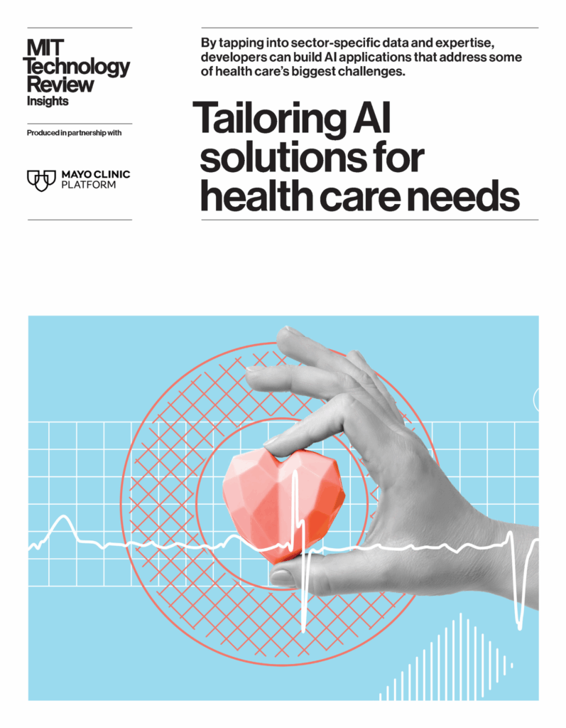
Tailoring AI solutions for health care needs

The AI market is full of big promises of grand transformation. Health care is a prime target for those promises, beset as it is by financial pressures, labor shortages, and the growing burden of caring for an aging population. AI developers are targeting functions that vary widely, from curing cancer and performing surgery to streamlining routine administrative tasks. The opportunity is genuine, but execution can be difficult. Numerous software vendors have tried to “fix” health care challenges but failed because they misunderstood the environment. “Health care is very complex,” says Steve Bethke, vice president of the solution developer market for Mayo Clinic Platform, which supports the buildout and deployment of digital solutions for health care companies through data-based insights and expert validation. “Solution developers must have a deep focus on clinical and technical capabilities, and then align their solutions to the relevant business impacts. If they miss any dimension, the solution will not be adopted or drive value.” DOWNLOAD THE REPORT AI applications for health care are proliferating rapidly. The U.S. Food and Drug Administration has approved more than 1,300 AI-enabled medical devices, mostly for interpreting diagnostic images. More than half of these were approved in the past three years, with the earliest dating as far back as 1995. Non-radiological applications carry out tasks as diverse as tracking sleep apnea, analyzing heart rhythms, and planning orthopedic surgeries. AI applications that do not count as medical devices— for example, those that handle scheduling and administrative tasks—are more difficult to track but are also rapidly increasing. AI can help coordinate complex tasks and workflows that are often conventionally managed by whiteboards and sticky notes. Such functions may well outstrip clinical uses in their impact on health systems. A recent survey of technology leaders found that 72% said their top priority for AI was reducing caregiver burden and improving caregiver satisfaction, while over half (53%) cited workflow efficiency and productivity. Any health care-related application can potentially impact patient care, whether directly or indirectly, and AI apps that are poorly designed or inadequately trained and validated can put patients at risk. Providers recognize that risk: In the same survey, 77% said immature AI tools are a significant barrier to adoption. Regulators and lawmakers are also keeping an eye on the risks as development and adoption burgeon, though the U.S. regulatory picture is still in flux, as a 2024 report to Congress on AI in health care observes. To tackle some of the technical challenges, many health care providers are partnering with application developers to build AI solutions. In a recent study, McKinsey found that 61% of health care organizations intend to pursue partnerships with third-party vendors to develop customized generative AI solutions as a primary strategy as opposed to building them in-house or buying off-the-shelf products. But health care-specific AI applications must also be tailored to the nuanced clinical needs of medical providers as well as the complex business and regulatory considerations of the wider sector. This is where developers can benefit from working with a partner with a deep understanding of the health care environment to tailor applications to what providers want and need most. Doing so helps to position AI products for maximum impact and value, avoiding the pitfalls unique to the health care environment. Download the report. This content was produced by Insights, the custom content arm of MIT Technology Review. It was not written by MIT Technology Review’s editorial staff. It was researched, designed, and written by human writers, editors, analysts, and illustrators. This includes the writing of surveys and collection of data for surveys. AI tools that may have been used were limited to secondary production processes that passed thorough human review.

Tailoring AI solutions for health care needs Leggi l'articolo »

AI, Committee, Notizie, Uncategorized

Build a Multi-Agent AI Workflow for Biological Network Modeling, Protein Interactions, Metabolism, and Cell Signaling Simulation

In this tutorial, we build a multi-agent workflow for biological systems modeling and explore how different computational components work together inside one unified systems biology pipeline. We generate synthetic biological data, analyze gene regulatory structure, predict protein-protein interactions, optimize metabolic pathway activity, and simulate a dynamic cell signaling cascade, all within a Colab environment that remains practical and reproducible. We also use an OpenAI model to act as a principal investigator, synthesizing the outputs of all specialized agents into a single expert-style biological interpretation that connects regulation, interaction networks, metabolism, and signaling into a broader scientific story. Copy CodeCopiedUse a different Browser import sys, subprocess, pkgutil def _install_if_missing(packages): missing = [] for p in packages: import_name = p[“import”] if pkgutil.find_loader(import_name) is None: missing.append(p[“pip”]) if missing: print(“Installing:”, “, “.join(missing)) subprocess.check_call([sys.executable, “-m”, “pip”, “install”, “-q”] + missing) _install_if_missing([ {“pip”: “openai”, “import”: “openai”}, {“pip”: “numpy”, “import”: “numpy”}, {“pip”: “pandas”, “import”: “pandas”}, {“pip”: “matplotlib”, “import”: “matplotlib”}, {“pip”: “networkx”, “import”: “networkx”}, {“pip”: “scikit-learn”, “import”: “sklearn”}, ]) import os import json import math import textwrap import random import getpass from dataclasses import dataclass from typing import Dict, List, Tuple, Any import numpy as np import pandas as pd import matplotlib.pyplot as plt import networkx as nx from sklearn.linear_model import LogisticRegression from sklearn.metrics import roc_auc_score, average_precision_score from sklearn.model_selection import train_test_split from sklearn.preprocessing import StandardScaler from openai import OpenAI np.random.seed(42) random.seed(42) OPENAI_API_KEY = None try: from google.colab import userdata OPENAI_API_KEY = userdata.get(“OPENAI_API_KEY”) if OPENAI_API_KEY: print(“Loaded OPENAI_API_KEY from Colab Secrets.”) except Exception: pass if not OPENAI_API_KEY: try: OPENAI_API_KEY = getpass.getpass(“Enter OPENAI_API_KEY (hidden input): “).strip() except Exception: OPENAI_API_KEY = input(“Enter OPENAI_API_KEY: “).strip() os.environ[“OPENAI_API_KEY”] = OPENAI_API_KEY client = OpenAI(api_key=OPENAI_API_KEY) OPENAI_MODEL = “gpt-4o-mini” We prepare the Colab environment and make sure all required libraries are available before the workflow begins. We import the scientific computing, machine learning, graph analysis, plotting, and OpenAI libraries that support the full biological systems pipeline from start to finish. We also securely load the OpenAI API key either from Colab Secrets or hidden input, initialize the client, and define the model so the notebook is ready for later LLM-based synthesis. Copy CodeCopiedUse a different Browser def sigmoid(x): return 1 / (1 + np.exp(-x)) def pretty(title: str, body: str, width: int = 100): print(“n” + “=” * width) print(title) print(“=” * width) print(body) def safe_float(x): try: return float(x) except Exception: return None def generate_gene_regulatory_network(n_genes: int = 14, edge_prob: float = 0.18): genes = [f”G{i+1}” for i in range(n_genes)] W = np.zeros((n_genes, n_genes)) for i in range(n_genes): for j in range(n_genes): if i != j and np.random.rand() < edge_prob: W[i, j] = np.random.uniform(-1.5, 1.5) return genes, W def simulate_gene_expression(W: np.ndarray, n_steps: int = 70, noise: float = 0.10): n = W.shape[0] X = np.zeros((n_steps, n)) X[0] = np.random.uniform(0.2, 0.8, size=n) for t in range(1, n_steps): signal = X[t-1] @ W X[t] = sigmoid(signal + np.random.normal(0, noise, size=n)) return X def generate_protein_features(n_proteins: int = 40, feature_dim: int = 10): proteins = [f”P{i+1}” for i in range(n_proteins)] features = np.random.normal(size=(n_proteins, feature_dim)) families = np.random.randint(0, 5, size=n_proteins) localization = np.random.randint(0, 4, size=n_proteins) return proteins, features, families, localization def generate_ppi_dataset(proteins, features, families, localization): rows = [] n = len(proteins) hidden_w = np.random.normal(size=features.shape[1]) for i in range(n): for j in range(i + 1, n): fi, fj = features[i], features[j] sim = np.dot(fi, fj) / (np.linalg.norm(fi) * np.linalg.norm(fj) + 1e-8) fam_same = 1 if families[i] == families[j] else 0 loc_same = 1 if localization[i] == localization[j] else 0 feat = np.concatenate([ np.abs(fi – fj), fi * fj, [sim, fam_same, loc_same] ]) score = 1.4 * sim + 1.0 * fam_same + 0.8 * loc_same + 0.15 * np.dot((fi + fj) / 2, hidden_w) prob = sigmoid(score) y = 1 if np.random.rand() < prob else 0 rows.append((proteins[i], proteins[j], feat, y)) return rows def generate_metabolic_network(): metabolites = [“Glucose”, “Pyruvate”, “AcetylCoA”, “ATP”, “Biomass”, “Lactate”, “Ethanol”] reactions = [ {“name”: “R1_Glucose_Uptake”, “yield_biomass”: 0.0, “yield_atp”: 0.3, “substrate_cost”: 1.0, “oxygen_need”: 0.0}, {“name”: “R2_Glycolysis”, “yield_biomass”: 0.2, “yield_atp”: 1.6, “substrate_cost”: 0.7, “oxygen_need”: 0.0}, {“name”: “R3_TCA”, “yield_biomass”: 1.0, “yield_atp”: 2.4, “substrate_cost”: 0.8, “oxygen_need”: 1.4}, {“name”: “R4_Fermentation”, “yield_biomass”: 0.1, “yield_atp”: 0.9, “substrate_cost”: 0.4, “oxygen_need”: 0.0}, {“name”: “R5_Ethanol_Path”, “yield_biomass”: 0.15,”yield_atp”: 0.8, “substrate_cost”: 0.5, “oxygen_need”: 0.0}, {“name”: “R6_Biomass_Assembly”,”yield_biomass”: 1.3, “yield_atp”: -0.9,”substrate_cost”: 0.6, “oxygen_need”: 0.2}, ] return metabolites, reactions def simulate_cell_signaling(T=200, dt=0.05, ligand_level=1.2): t = np.arange(0, T * dt, dt) ligand = np.ones_like(t) * ligand_level receptor = np.zeros_like(t) kinase = np.zeros_like(t) tf = np.zeros_like(t) phosphatase = np.zeros_like(t) receptor[0] = 0.05 kinase[0] = 0.02 tf[0] = 0.01 phosphatase[0] = 0.30 for i in range(1, len(t)): dR = 1.6 * ligand[i-1] * (1 – receptor[i-1]) – 0.9 * receptor[i-1] dK = 1.8 * receptor[i-1] * (1 – kinase[i-1]) – 1.1 * phosphatase[i-1] * kinase[i-1] dTF = 1.4 * kinase[i-1] * (1 – tf[i-1]) – 0.55 * tf[i-1] dP = 0.2 + 0.5 * tf[i-1] – 0.4 * phosphatase[i-1] receptor[i] = np.clip(receptor[i-1] + dt * dR, 0, 1) kinase[i] = np.clip(kinase[i-1] + dt * dK, 0, 1) tf[i] = np.clip(tf[i-1] + dt * dTF, 0, 1) phosphatase[i] = np.clip(phosphatase[i-1] + dt * dP, 0, 1.5) return pd.DataFrame({ “time”: t, “ligand”: ligand, “receptor_active”: receptor, “kinase_active”: kinase, “tf_active”: tf, “phosphatase”: phosphatase, }) We define the main helper utilities and all synthetic data generation functions that power the notebook’s biological tasks. We create functions for gene regulatory network construction, gene expression simulation, protein feature generation, protein interaction dataset creation, metabolic network setup, and cell signaling dynamics, which together provide four distinct biological views for analysis. This snippet forms the computational backbone of the tutorial by creating the structured inputs that each specialized agent will later process and interpret. Copy CodeCopiedUse a different Browser @dataclass class AgentResult: name: str summary: Dict[str, Any] class GeneRegulatoryNetworkAgent: def run(self, genes, W, X) -> AgentResult: corr = np.corrcoef(X.T) inferred_edges = [] true_edges = [] n = len(genes) for i in range(n): for j in range(n): if i == j: continue if abs(corr[i, j]) > 0.35: inferred_edges.append((genes[i], genes[j], float(corr[i, j]))) if abs(W[i, j]) > 1e-8: true_edges.append((genes[i], genes[j], float(W[i, j]))) centrality_graph = nx.DiGraph() for gi in genes: centrality_graph.add_node(gi) for i in range(n): for j in range(n): if abs(W[i, j]) >

Build a Multi-Agent AI Workflow for Biological Network Modeling, Protein Interactions, Metabolism, and Cell Signaling Simulation Leggi l'articolo »

AI, Committee, Notizie, Uncategorized

Mistral AI Launches Remote Agents in Vibe and Mistral Medium 3.5 with 77.6% SWE-Bench Verified Score

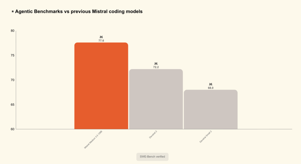
Mistral AI has been quietly building one of the more practical coding agent ecosystems in the open-source/weights AI space, and they are shipping its most significant infrastructure upgrade yet. Mistral team announced remote agents in Vibe, its coding agent platform, alongside the public preview of Mistral Medium 3.5 — a new 128B dense model that now serves as the default model in both Vibe and Le Chat, Mistral’s consumer assistant. What is Vibe, and Why Does It Matter? If you haven’t used it yet, Mistral Vibe is a coding agent accessible through a CLI (command-line interface) that lets an AI model work through software tasks on your behalf — writing code, refactoring modules, generating tests, investigating CI failures, and more. Think of it as a junior developer that never gets tired and can operate across your codebase. Until now, Vibe sessions ran locally, meaning the agent was tied to your laptop and your terminal. That changes today. Remote Agents: The Agent Runs While You Step Away So, basically now coding sessions can work through long tasks while you’re away. Many can run in parallel, and you stop being the bottleneck on every step the agent takes. This is the key behavioral shift. Instead of babysitting a coding session in your terminal, you kick off a task and let the cloud handle the rest. You can start cloud agents from the Mistral Vibe CLI or from Le Chat. While they run, you can inspect what the agent is doing, with file diffs, tool calls, progress states, and questions surfaced as you go. One particularly useful feature for developers already mid-session: ongoing local CLI sessions can be teleported up to the cloud when you want to leave them running, with session history, task state, and approvals carrying across. So you don’t lose your place — you just move the work off your machine. Each session runs in isolation. Each coding session runs in an isolated sandbox, including broad edits and installs. When the work is done, the agent can open a pull request on GitHub and notify you, so you review the result instead of every keystroke that produced it. It’s also worth understanding the logic behind how Vibe connects to Le Chat. Mistral uses Workflows orchestrated in Mistral Studio to bring Mistral Vibe into Le Chat — originally built for their own in-house coding environment, then for enterprise customers, and now open to everyone. This means the remote coding agent in Le Chat is not a standalone feature — it’s built on top of Mistral’s own orchestration layer, which is useful context if you’re thinking about how to architect similar agentic systems yourself. On the integration side, Vibe plugs into GitHub for code and pull requests, Linear and Jira for issues, Sentry for incidents, and apps like Slack or Teams for reporting. Mistral Medium 3.5: The Model Behind It All None of this would be practically possible without a capable underlying AI model. This new released model is Mistral Medium 3.5, which Mistral team describes as its first flagship merged model. It is a dense 128B model with a 256k context window, handling instruction-following, reasoning, and coding in a single set of weights. For context, a 256k context window means the model can process roughly 200,000 words in a single pass — long enough to reason across an entire large codebase. The model is also multimodal. Mistral team trained the vision encoder from scratch to handle variable image sizes and aspect ratios — a notable architectural choice. Most vision-language models reuse pretrained encoders like CLIP, so building this component from scratch suggests Mistral prioritized flexibility in how the model handles real-world image inputs rather than defaulting to fixed-resolution assumptions. Mistral Medium 3.5 scores 77.6% on SWE-Bench Verified, ahead of Devstral 2 and models like Qwen3.5 397B A17B. SWE-Bench Verified is a standard benchmark that tests whether a model can resolve real-world GitHub issues from popular open-source repositories — it’s one of the most reliable proxies for practical software engineering ability. The model also scores 91.4 on τ³-Telecom and has strong agentic capabilities. https://mistral.ai/news/vibe-remote-agents-mistral-medium-3-5 One particularly interesting design choice: reasoning effort is now configurable per request, so the same model can answer a quick chat reply or work through a complex agentic run. This is important for developers integrating the model via API — you can dial down compute for simple lookups and dial it up for multi-step reasoning tasks, without switching models. The model was built for long-horizon tasks, calling multiple tools reliably, and producing structured output that downstream code can consume. Work Mode in Le Chat: A New Agentic Layer Beyond the coding agent upgrades, Mistral is also shipping Work mode in Le Chat — a new agentic mode for more general, multi-step tasks. Work mode is a powerful new agentic mode for complex tasks in Le Chat, powered by a new harness and Mistral Medium 3.5. The agent becomes the execution backend for the assistant itself, so Le Chat can read and write, use several tools at once, and work through multi-step projects until it completes what you’ve asked. Practically, this means things like cross-tool workflows — catching up across email, messages, and calendar; preparing for a meeting with relevant context pulled from multiple sources; or triaging an inbox and creating Jira issues from team discussions. In Work mode, connectors are on by default rather than chosen manually, which lets the agent reach into documents, mailboxes, calendars, and other systems for the rich context it needs to take correct action. This is a significant usability shift from typical chat assistants, where you manually select tools before each session. Transparency is a built-in feature rather than an afterthought: every action the agent takes is visible — you see each tool call and the thinking rationale. Le Chat will ask for explicit approval — based on your permissions — before proceeding with sensitive tasks like sending a message, writing a document, or modifying data. Key Takeaways Here are the key

Mistral AI Launches Remote Agents in Vibe and Mistral Medium 3.5 with 77.6% SWE-Bench Verified Score Leggi l'articolo »

We use cookies to improve your experience and performance on our website. You can learn more at Politica sulla privacy and manage your privacy settings by clicking Settings.

Privacy Preferences

You can choose your cookie settings by turning on/off each type of cookie as you wish, except for essential cookies.

Allow All
Manage Consent Preferences
  • Always Active

Save
it_IT