YouZum

Uncategorized

AI, Committee, Actualités, Uncategorized

Multimodal LLMs Do Not Compose Skills Optimally Across Modalities

arXiv:2511.08113v1 Announce Type: new Abstract: Skill composition is the ability to combine previously learned skills to solve new tasks. As neural networks acquire increasingly complex skills during their pretraining, it is not clear how successfully they can compose them. In this paper, we focus on Multimodal Large Language Models (MLLM), and study their ability to compose skills across modalities. To this end, we design three evaluation tasks which can be solved sequentially composing two modality-dependent skills, and evaluate several open MLLMs under two main settings: i) prompting the model to directly solve the task, and ii) using a two-step cascaded inference approach, which manually enforces the composition of the two skills for a given task. Even with these straightforward compositions, we find that all evaluated MLLMs exhibit a significant cross-modality skill composition gap. To mitigate the aforementioned gap, we explore two alternatives: i) use chain-of-thought prompting to explicitly instruct MLLMs for skill composition and ii) a specific fine-tuning recipe to promote skill composition. Although those strategies improve model performance, they still exhibit significant skill composition gaps, suggesting that more research is needed to improve cross-modal skill composition in MLLMs.

Multimodal LLMs Do Not Compose Skills Optimally Across Modalities Lire l’article »

AI, Committee, Actualités, Uncategorized

Baidu Releases ERNIE-4.5-VL-28B-A3B-Thinking: An Open-Source and Compact Multimodal Reasoning Model Under the ERNIE-4.5 Family

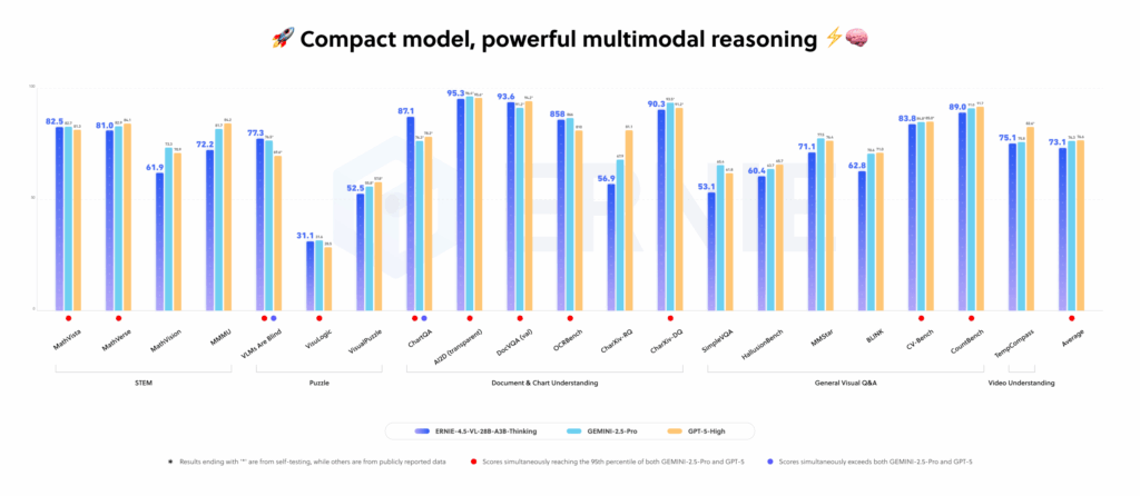
How can we get large model level multimodal reasoning for documents, charts and videos while running only a 3B class model in production? Baidu has added a new model to the ERNIE-4.5 open source family. ERNIE-4.5-VL-28B-A3B-Thinking is a vision language model that focuses on document, chart and video understanding with a small active parameter budget. https://huggingface.co/baidu/ERNIE-4.5-VL-28B-A3B-Thinking Architecture and training setup ERNIE-4.5-VL-28B-A3B-Thinking is built on the ERNIE-4.5-VL-28B-A3B Mixture of Experts architecture. The family uses a heterogeneous multimodal MoE design with shared parameters across text and vision plus modality specific experts. At the model level, it has 30B total parameters, while the architecture is in the 28B-VL branch, and only 3B parameters are activated per token through an A3B routing scheme. This gives the compute and memory profile of a 3B class model while keeping a larger capacity pool for reasoning. The model goes through an additional mid training stage on a large visual language reasoning corpus. This stage is designed to improve representation power and semantic alignment between visual and language modalities, which matters for dense text in documents and fine structures in charts. On top of that, ERNIE-4.5-VL-28B-A3B-Thinking uses multimodal reinforcement learning on verifiable tasks, with GSPO and IcePop strategies and dynamic difficulty sampling to stabilize MoE training and push the model toward hard examples. Key capabilities Baidu researchers position this model as a lightweight multimodal reasoning engine that can activate only 3B parameters while approaching the behavior of larger flagship systems on internal benchmarks. Officially listed capabilities include visual reasoning, STEM reasoning, visual grounding, Thinking with Images, tool utilization and video understanding. Thinking with Images is at the core. The model can zoom into regions, reason on cropped views and then integrate those local observations into a final answer. Tool utilization extends this with calls to tools such as image search when internal knowledge is not enough. Both features are exposed as part of the reasoning parser and tool call parser path in deployment. Performance and positioning The lightweight vision language model ERNIE-4.5-VL-28B-A3B achieves competitive or superior performance compared to Qwen-2.5-VL-7B and Qwen-2.5-VL-32B on many benchmarks, while using fewer activation parameters. ERNIE-4.5-VL models also support both thinking and non thinking modes, with the thinking mode improving reasoning centered tasks while keeping strong perception quality. For the specific Thinking variant, Baidu researchers describe ERNIE-4.5-VL-28B-A3B-Thinking as closely matching the performance of industry flagship models across internal multimodal benchmarks. Key Takeaways ERNIE-4.5-VL-28B-A3B-Thinking uses a Mixture of Experts architecture with about 30B total parameters and only 3B active parameters per token to deliver efficient multimodal reasoning. The model is optimized for document, chart and video understanding through an additional visual language reasoning mid training stage and multimodal reinforcement learning using GSPO, IcePop and dynamic difficulty sampling. Thinking with Images lets the model iteratively zoom into image regions and reason over crops, while tool utilization enables calls to external tools such as image search for long tail recognition. It demonstrate strong performance on analytics style charts, STEM circuit problems, visual grounding with JSON bounding boxes and video segment localization with timestamped answers. The model is released under Apache License 2.0, supports deployment via transformers, vLLM and FastDeploy, and can be fine tuned with ERNIEKit using SFT, LoRA and DPO for commercial multimodal applications. Comparison Table Model Training stage Total / active parameters Modalities Context length (tokens) ERNIE-4.5-VL-28B-A3B-Base Pretraining 28B total, 3B active per token Text, Vision 131,072 ERNIE-4.5-VL-28B-A3B (PT) Posttraining chat model 28B total, 3B active per token Text, Vision 131,072 ERNIE-4.5-VL-28B-A3B-Thinking Reasoning oriented mid training on ERNIE-4.5-VL-28B-A3B 28B architecture, 3B active per token, HF model size 30B params Text, Vision 131,072 (FastDeploy example uses 131,072 max model length) Qwen2.5-VL-7B-Instruct Posttraining vision language model ≈8B total (7B class) Text, Image, Video 32,768 text positions in config (max_position_embeddings) Qwen2.5-VL-32B-Instruct Posttraining plus reinforcement tuned large VL model 33B total Text, Image, Video 32,768 text positions (same Qwen2.5-VLTextConfig family) Editorial Comments ERNIE-4.5-VL-28B-A3B-Thinking is a practical release for teams that want multimodal reasoning on documents, charts and videos with only 3B activated parameters, while still using a Mixture-of-Experts architecture with about 30B total parameters and Apache License 2.0. It connects Thinking with Images, tool utilization and multimodal reinforcement learning into a deployable stack that directly targets real world analytics and understanding workloads. Check out the Repo, Model Weights and Technical details. Feel free to check out our GitHub Page for Tutorials, Codes and Notebooks. Also, feel free to follow us on Twitter and don’t forget to join our 100k+ ML SubReddit and Subscribe to our Newsletter. Wait! are you on telegram? now you can join us on telegram as well. The post Baidu Releases ERNIE-4.5-VL-28B-A3B-Thinking: An Open-Source and Compact Multimodal Reasoning Model Under the ERNIE-4.5 Family appeared first on MarkTechPost.

Baidu Releases ERNIE-4.5-VL-28B-A3B-Thinking: An Open-Source and Compact Multimodal Reasoning Model Under the ERNIE-4.5 Family Lire l’article »

AI, Committee, Actualités, Uncategorized

How to Build an End-to-End Interactive Analytics Dashboard Using PyGWalker Features for Insightful Data Exploration

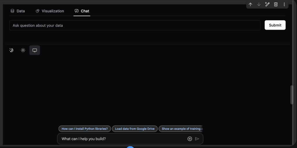
In this tutorial, we explore the advanced capabilities of PyGWalker, a powerful tool for visual data analysis that integrates seamlessly with pandas. We begin by generating a realistic e-commerce dataset enriched with time, demographic, and marketing features to mimic real-world business data. We then prepare multiple analytical views, including daily sales, category performance, and customer segment summaries. Finally, we use PyGWalker to interactively explore patterns, correlations, and trends across these dimensions through intuitive drag-and-drop visualizations. Check out the FULL CODES here. Copy CodeCopiedUse a different Browser !pip install pygwalker pandas numpy scikit-learn import pandas as pd import numpy as np import pygwalker as pyg from datetime import datetime, timedelta We begin by setting up our environment, installing all necessary dependencies, and importing essential libraries, including pandas, numpy, and pygwalker. We ensure that everything is ready for building our interactive data exploration workflow in Colab. Check out the FULL CODES here. Copy CodeCopiedUse a different Browser def generate_advanced_dataset(): np.random.seed(42) start_date = datetime(2022, 1, 1) dates = [start_date + timedelta(days=x) for x in range(730)] categories = [‘Electronics’, ‘Clothing’, ‘Home & Garden’, ‘Sports’, ‘Books’] products = { ‘Electronics’: [‘Laptop’, ‘Smartphone’, ‘Headphones’, ‘Tablet’, ‘Smartwatch’], ‘Clothing’: [‘T-Shirt’, ‘Jeans’, ‘Dress’, ‘Jacket’, ‘Sneakers’], ‘Home & Garden’: [‘Furniture’, ‘Lamp’, ‘Rug’, ‘Plant’, ‘Cookware’], ‘Sports’: [‘Yoga Mat’, ‘Dumbbell’, ‘Running Shoes’, ‘Bicycle’, ‘Tennis Racket’], ‘Books’: [‘Fiction’, ‘Non-Fiction’, ‘Biography’, ‘Science’, ‘History’] } n_transactions = 5000 data = [] for _ in range(n_transactions): date = np.random.choice(dates) category = np.random.choice(categories) product = np.random.choice(products[category]) base_prices = { ‘Electronics’: (200, 1500), ‘Clothing’: (20, 150), ‘Home & Garden’: (30, 500), ‘Sports’: (25, 300), ‘Books’: (10, 50) } price = np.random.uniform(*base_prices[category]) quantity = np.random.choice([1, 1, 1, 2, 2, 3], p=[0.5, 0.2, 0.15, 0.1, 0.03, 0.02]) customer_segment = np.random.choice([‘Premium’, ‘Standard’, ‘Budget’], p=[0.2, 0.5, 0.3]) age_group = np.random.choice([’18-25′, ’26-35′, ’36-45′, ’46-55′, ’56+’]) region = np.random.choice([‘North’, ‘South’, ‘East’, ‘West’, ‘Central’]) month = date.month seasonal_factor = 1.0 if month in [11, 12]: seasonal_factor = 1.5 elif month in [6, 7]: seasonal_factor = 1.2 revenue = price * quantity * seasonal_factor discount = np.random.choice([0, 5, 10, 15, 20, 25], p=[0.4, 0.2, 0.15, 0.15, 0.07, 0.03]) marketing_channel = np.random.choice([‘Organic’, ‘Social Media’, ‘Email’, ‘Paid Ads’]) base_satisfaction = 4.0 if customer_segment == ‘Premium’: base_satisfaction += 0.5 if discount > 15: base_satisfaction += 0.3 satisfaction = np.clip(base_satisfaction + np.random.normal(0, 0.5), 1, 5) data.append({ ‘Date’: date, ‘Category’: category, ‘Product’: product, ‘Price’: round(price, 2), ‘Quantity’: quantity, ‘Revenue’: round(revenue, 2), ‘Customer_Segment’: customer_segment, ‘Age_Group’: age_group, ‘Region’: region, ‘Discount_%’: discount, ‘Marketing_Channel’: marketing_channel, ‘Customer_Satisfaction’: round(satisfaction, 2), ‘Month’: date.strftime(‘%B’), ‘Year’: date.year, ‘Quarter’: f’Q{(date.month-1)//3 + 1}’ }) df = pd.DataFrame(data) df[‘Profit_Margin’] = round(df[‘Revenue’] * (1 – df[‘Discount_%’]/100) * 0.3, 2) df[‘Days_Since_Start’] = (df[‘Date’] – df[‘Date’].min()).dt.days return df We design a function to generate a comprehensive e-commerce dataset that mirrors real-world business conditions. We include product categories, customer demographics, seasonal effects, and satisfaction levels, ensuring that our data is diverse and analytically rich. Check out the FULL CODES here. Copy CodeCopiedUse a different Browser print(“Generating advanced e-commerce dataset…”) df = generate_advanced_dataset() print(f”nDataset Overview:”) print(f”Total Transactions: {len(df)}”) print(f”Date Range: {df[‘Date’].min()} to {df[‘Date’].max()}”) print(f”Total Revenue: ${df[‘Revenue’].sum():,.2f}”) print(f”nColumns: {list(df.columns)}”) print(“nFirst few rows:”) print(df.head()) We execute the dataset generation function and display key insights, including total transactions, revenue range, and sample records. We get a clear snapshot of the data’s structure and confirm that it’s suitable for detailed analysis. Check out the FULL CODES here. Copy CodeCopiedUse a different Browser daily_sales = df.groupby(‘Date’).agg({ ‘Revenue’: ‘sum’, ‘Quantity’: ‘sum’, ‘Customer_Satisfaction’: ‘mean’ }).reset_index() category_analysis = df.groupby(‘Category’).agg({ ‘Revenue’: [‘sum’, ‘mean’], ‘Quantity’: ‘sum’, ‘Customer_Satisfaction’: ‘mean’, ‘Profit_Margin’: ‘sum’ }).reset_index() category_analysis.columns = [‘Category’, ‘Total_Revenue’, ‘Avg_Order_Value’, ‘Total_Quantity’, ‘Avg_Satisfaction’, ‘Total_Profit’] segment_analysis = df.groupby([‘Customer_Segment’, ‘Region’]).agg({ ‘Revenue’: ‘sum’, ‘Customer_Satisfaction’: ‘mean’ }).reset_index() print(“n” + “=”*50) print(“DATASET READY FOR PYGWALKER VISUALIZATION”) print(“=”*50) We perform data aggregations to prepare multiple analytical perspectives, including time-based trends, category-level summaries, and performance metrics for customer segments. We organize this information to make it easily visualizable in PyGWalker. Check out the FULL CODES here. Copy CodeCopiedUse a different Browser print(“n Launching PyGWalker Interactive Interface…”) walker = pyg.walk( df, spec=”./pygwalker_config.json”, use_kernel_calc=True, theme_key=’g2′ ) print(“n PyGWalker is now running!”) print(” Try creating these visualizations:”) print(” – Revenue trend over time (line chart)”) print(” – Category distribution (pie chart)”) print(” – Price vs Satisfaction scatter plot”) print(” – Regional sales heatmap”) print(” – Discount effectiveness analysis”) We launch the PyGWalker interactive interface to visually explore our dataset. We create meaningful charts, uncover trends in sales, satisfaction, and pricing, and observe how interactive visualization enhances our analytical understanding. Data View Visualization Chat with Data In conclusion, we developed a comprehensive data visualization workflow using PyGWalker, encompassing dataset generation, feature engineering, multidimensional analysis, and interactive exploration. We experience how PyGWalker transforms raw tabular data into rich, exploratory dashboards without needing complex code or BI tools. Through this exercise, we strengthen our ability to derive insights quickly, experiment visually, and connect data storytelling directly to practical business understanding. Check out the FULL CODES here. Feel free to check out our GitHub Page for Tutorials, Codes and Notebooks. Also, feel free to follow us on Twitter and don’t forget to join our 100k+ ML SubReddit and Subscribe to our Newsletter. Wait! are you on telegram? now you can join us on telegram as well. The post How to Build an End-to-End Interactive Analytics Dashboard Using PyGWalker Features for Insightful Data Exploration appeared first on MarkTechPost.

How to Build an End-to-End Interactive Analytics Dashboard Using PyGWalker Features for Insightful Data Exploration Lire l’article »

AI, Committee, Actualités, Uncategorized

Adapting Web Agents with Synthetic Supervision

arXiv:2511.06101v1 Announce Type: cross Abstract: Web agents struggle to adapt to new websites due to the scarcity of environment specific tasks and demonstrations. Recent works have explored synthetic data generation to address this challenge, however, they suffer from data quality issues where synthesized tasks contain hallucinations that cannot be executed, and collected trajectories are noisy with redundant or misaligned actions. In this paper, we propose SynthAgent, a fully synthetic supervision framework that aims at improving synthetic data quality via dual refinement of both tasks and trajectories. Our approach begins by synthesizing diverse tasks through categorized exploration of web elements, ensuring efficient coverage of the target environment. During trajectory collection, we refine tasks when conflicts with actual observations are detected, mitigating hallucinations while maintaining task consistency. After collection, we conduct trajectory refinement with a global context to mitigate potential noise or misalignments. Finally, we fine-tune open-source web agents on the refined synthetic data to adapt them to the target environment. Experimental results demonstrate that SynthAgent outperforms existing synthetic data methods, validating the importance of high-quality synthetic supervision. The code will be publicly available at https://github.com/aiming-lab/SynthAgent.

Adapting Web Agents with Synthetic Supervision Lire l’article »

AI, Committee, Actualités, Uncategorized

Rethinking Tokenization for Rich Morphology: The Dominance of Unigram over BPE and Morphological Alignment

arXiv:2508.08424v3 Announce Type: replace Abstract: The relationship between tokenizer algorithm (e.g., Byte-Pair Encoding (BPE), Unigram), morphological alignment, tokenization quality (e.g., compression efficiency), and downstream performance remains largely unclear, particularly for languages with complex morphology. In this paper, we conduct a comprehensive evaluation of tokenizers using small-sized BERT models — from pre-training through fine-tuning — for Telugu (agglutinative), along with preliminary evaluation in Hindi (primarily fusional with some agglutination) and English (fusional). To evaluate morphological alignment of tokenizers in Telugu, we create a dataset containing gold morpheme segmentations of 600 derivational and 7000 inflectional word forms. Our experiments reveal two key findings for Telugu. First, the choice of tokenizer algorithm is the most significant factor influencing performance, with Unigram-based tokenizers consistently outperforming BPE across most settings. Second, while better morphological alignment shows a moderate, positive correlation with performance on text classification and structure prediction tasks, its impact is secondary to the tokenizer algorithm. Notably, hybrid approaches that use morphological information for pre-segmentation significantly boost the performance of BPE, though not Unigram. Our results further showcase the need for comprehensive intrinsic evaluation metrics for tokenizers that could explain downstream performance trends consistently.

Rethinking Tokenization for Rich Morphology: The Dominance of Unigram over BPE and Morphological Alignment Lire l’article »

AI, Committee, Actualités, Uncategorized

When AI Agents Collude Online: Financial Fraud Risks by Collaborative LLM Agents on Social Platforms

arXiv:2511.06448v1 Announce Type: cross Abstract: In this work, we study the risks of collective financial fraud in large-scale multi-agent systems powered by large language model (LLM) agents. We investigate whether agents can collaborate in fraudulent behaviors, how such collaboration amplifies risks, and what factors influence fraud success. To support this research, we present MultiAgentFraudBench, a large-scale benchmark for simulating financial fraud scenarios based on realistic online interactions. The benchmark covers 28 typical online fraud scenarios, spanning the full fraud lifecycle across both public and private domains. We further analyze key factors affecting fraud success, including interaction depth, activity level, and fine-grained collaboration failure modes. Finally, we propose a series of mitigation strategies, including adding content-level warnings to fraudulent posts and dialogues, using LLMs as monitors to block potentially malicious agents, and fostering group resilience through information sharing at the societal level. Notably, we observe that malicious agents can adapt to environmental interventions. Our findings highlight the real-world risks of multi-agent financial fraud and suggest practical measures for mitigating them. Code is available at https://github.com/zheng977/MutiAgent4Fraud.

When AI Agents Collude Online: Financial Fraud Risks by Collaborative LLM Agents on Social Platforms Lire l’article »

AI, Committee, Actualités, Uncategorized

A Coding Implementation to Build and Train Advanced Architectures with Residual Connections, Self-Attention, and Adaptive Optimization Using JAX, Flax, and Optax

In this tutorial, we explore how to build and train an advanced neural network using JAX, Flax, and Optax in an efficient and modular way. We begin by designing a deep architecture that integrates residual connections and self-attention mechanisms for expressive feature learning. As we progress, we implement sophisticated optimization strategies with learning rate scheduling, gradient clipping, and adaptive weight decay. Throughout the process, we leverage JAX transformations such as jit, grad, and vmap to accelerate computation and ensure smooth training performance across devices. Check out the FULL CODES here. Copy CodeCopiedUse a different Browser !pip install jax jaxlib flax optax matplotlib import jax import jax.numpy as jnp from jax import random, jit, vmap, grad import flax.linen as nn from flax.training import train_state import optax import matplotlib.pyplot as plt from typing import Any, Callable print(f”JAX version: {jax.__version__}”) print(f”Devices: {jax.devices()}”) We begin by installing and importing JAX, Flax, and Optax, along with essential utilities for numerical operations and visualization. We check our device setup to ensure that JAX is running efficiently on available hardware. This setup forms the foundation for the entire training pipeline. Check out the FULL CODES here. Copy CodeCopiedUse a different Browser class SelfAttention(nn.Module): num_heads: int dim: int @nn.compact def __call__(self, x): B, L, D = x.shape head_dim = D // self.num_heads qkv = nn.Dense(3 * D)(x) qkv = qkv.reshape(B, L, 3, self.num_heads, head_dim) q, k, v = jnp.split(qkv, 3, axis=2) q, k, v = q.squeeze(2), k.squeeze(2), v.squeeze(2) attn_scores = jnp.einsum(‘bhqd,bhkd->bhqk’, q, k) / jnp.sqrt(head_dim) attn_weights = jax.nn.softmax(attn_scores, axis=-1) attn_output = jnp.einsum(‘bhqk,bhvd->bhqd’, attn_weights, v) attn_output = attn_output.reshape(B, L, D) return nn.Dense(D)(attn_output) class ResidualBlock(nn.Module): features: int @nn.compact def __call__(self, x, training: bool = True): residual = x x = nn.Conv(self.features, (3, 3), padding=’SAME’)(x) x = nn.BatchNorm(use_running_average=not training)(x) x = nn.relu(x) x = nn.Conv(self.features, (3, 3), padding=’SAME’)(x) x = nn.BatchNorm(use_running_average=not training)(x) if residual.shape[-1] != self.features: residual = nn.Conv(self.features, (1, 1))(residual) return nn.relu(x + residual) class AdvancedCNN(nn.Module): num_classes: int = 10 @nn.compact def __call__(self, x, training: bool = True): x = nn.Conv(32, (3, 3), padding=’SAME’)(x) x = nn.relu(x) x = ResidualBlock(64)(x, training) x = ResidualBlock(64)(x, training) x = nn.max_pool(x, (2, 2), strides=(2, 2)) x = ResidualBlock(128)(x, training) x = ResidualBlock(128)(x, training) x = jnp.mean(x, axis=(1, 2)) x = x[:, None, :] x = SelfAttention(num_heads=4, dim=128)(x) x = x.squeeze(1) x = nn.Dense(256)(x) x = nn.relu(x) x = nn.Dropout(0.5, deterministic=not training)(x) x = nn.Dense(self.num_classes)(x) return x We define a deep neural network that combines residual blocks and a self-attention mechanism for enhanced feature learning. We construct the layers modularly, ensuring that the model can capture both spatial and contextual relationships. This design enables the network to generalize effectively across various types of input data. Check out the FULL CODES here. Copy CodeCopiedUse a different Browser class TrainState(train_state.TrainState): batch_stats: Any def create_learning_rate_schedule(base_lr: float = 1e-3, warmup_steps: int = 100, decay_steps: int = 1000) -> optax.Schedule: warmup_fn = optax.linear_schedule(init_value=0.0, end_value=base_lr, transition_steps=warmup_steps) decay_fn = optax.cosine_decay_schedule(init_value=base_lr, decay_steps=decay_steps, alpha=0.1) return optax.join_schedules(schedules=[warmup_fn, decay_fn], boundaries=[warmup_steps]) def create_optimizer(learning_rate_schedule: optax.Schedule) -> optax.GradientTransformation: return optax.chain(optax.clip_by_global_norm(1.0), optax.adamw(learning_rate=learning_rate_schedule, weight_decay=1e-4)) We create a custom training state that tracks model parameters and batch statistics. We also define a learning rate schedule with warmup and cosine decay, paired with an AdamW optimizer that includes gradient clipping and weight decay. This combination ensures stable and adaptive training. Check out the FULL CODES here. Copy CodeCopiedUse a different Browser @jit def compute_metrics(logits, labels): loss = optax.softmax_cross_entropy_with_integer_labels(logits, labels).mean() accuracy = jnp.mean(jnp.argmax(logits, -1) == labels) return {‘loss’: loss, ‘accuracy’: accuracy} def create_train_state(rng, model, input_shape, learning_rate_schedule): variables = model.init(rng, jnp.ones(input_shape), training=False) params = variables[‘params’] batch_stats = variables.get(‘batch_stats’, {}) tx = create_optimizer(learning_rate_schedule) return TrainState.create(apply_fn=model.apply, params=params, tx=tx, batch_stats=batch_stats) @jit def train_step(state, batch, dropout_rng): images, labels = batch def loss_fn(params): variables = {‘params’: params, ‘batch_stats’: state.batch_stats} logits, new_model_state = state.apply_fn(variables, images, training=True, mutable=[‘batch_stats’], rngs={‘dropout’: dropout_rng}) loss = optax.softmax_cross_entropy_with_integer_labels(logits, labels).mean() return loss, (logits, new_model_state) grad_fn = jax.value_and_grad(loss_fn, has_aux=True) (loss, (logits, new_model_state)), grads = grad_fn(state.params) state = state.apply_gradients(grads=grads, batch_stats=new_model_state[‘batch_stats’]) metrics = compute_metrics(logits, labels) return state, metrics @jit def eval_step(state, batch): images, labels = batch variables = {‘params’: state.params, ‘batch_stats’: state.batch_stats} logits = state.apply_fn(variables, images, training=False) return compute_metrics(logits, labels) We implement JIT-compiled training and evaluation functions to achieve efficient execution. The training step computes gradients, updates parameters, and dynamically maintains batch statistics. We also define evaluation metrics that help us monitor loss and accuracy throughout the training process. Check out the FULL CODES here. Copy CodeCopiedUse a different Browser def generate_synthetic_data(rng, num_samples=1000, img_size=32): rng_x, rng_y = random.split(rng) images = random.normal(rng_x, (num_samples, img_size, img_size, 3)) labels = random.randint(rng_y, (num_samples,), 0, 10) return images, labels def create_batches(images, labels, batch_size=32): num_batches = len(images) // batch_size for i in range(num_batches): idx = slice(i * batch_size, (i + 1) * batch_size) yield images[idx], labels[idx] We generate synthetic data to simulate an image classification task, enabling us to train the model without relying on external datasets. We then batch the data efficiently for iterative updates. This approach allows us to test the full pipeline quickly and verify that all components function correctly. Check out the FULL CODES here. Copy CodeCopiedUse a different Browser def train_model(num_epochs=5, batch_size=32): rng = random.PRNGKey(0) rng, data_rng, model_rng = random.split(rng, 3) train_images, train_labels = generate_synthetic_data(data_rng, num_samples=1000) test_images, test_labels = generate_synthetic_data(data_rng, num_samples=200) model = AdvancedCNN(num_classes=10) lr_schedule = create_learning_rate_schedule(base_lr=1e-3, warmup_steps=50, decay_steps=500) state = create_train_state(model_rng, model, (1, 32, 32, 3), lr_schedule) history = {‘train_loss’: [], ‘train_acc’: [], ‘test_acc’: []} print(“Starting training…”) for epoch in range(num_epochs): train_metrics = [] for batch in create_batches(train_images, train_labels, batch_size): rng, dropout_rng = random.split(rng) state, metrics = train_step(state, batch, dropout_rng) train_metrics.append(metrics) train_loss = jnp.mean(jnp.array([m[‘loss’] for m in train_metrics])) train_acc = jnp.mean(jnp.array([m[‘accuracy’] for m in train_metrics])) test_metrics = [eval_step(state, batch) for batch in create_batches(test_images, test_labels, batch_size)] test_acc = jnp.mean(jnp.array([m[‘accuracy’] for m in test_metrics])) history[‘train_loss’].append(float(train_loss)) history[‘train_acc’].append(float(train_acc)) history[‘test_acc’].append(float(test_acc)) print(f”Epoch {epoch + 1}/{num_epochs}: Loss: {train_loss:.4f}, Train Acc: {train_acc:.4f}, Test Acc: {test_acc:.4f}”) return history, state history, trained_state = train_model(num_epochs=5) fig, (ax1, ax2) = plt.subplots(1, 2, figsize=(12, 4)) ax1.plot(history[‘train_loss’], label=’Train Loss’) ax1.set_xlabel(‘Epoch’); ax1.set_ylabel(‘Loss’); ax1.set_title(‘Training Loss’); ax1.legend(); ax1.grid(True) ax2.plot(history[‘train_acc’], label=’Train Accuracy’) ax2.plot(history[‘test_acc’], label=’Test Accuracy’) ax2.set_xlabel(‘Epoch’); ax2.set_ylabel(‘Accuracy’); ax2.set_title(‘Model Accuracy’); ax2.legend(); ax2.grid(True) plt.tight_layout(); plt.show() print(“n Tutorial complete! This covers:”) print(“- Custom Flax modules (ResNet blocks, Self-Attention)”) print(“- Advanced Optax optimizers (AdamW with gradient clipping)”)

A Coding Implementation to Build and Train Advanced Architectures with Residual Connections, Self-Attention, and Adaptive Optimization Using JAX, Flax, and Optax Lire l’article »

AI, Committee, Actualités, Uncategorized

Rep2Text: Decoding Full Text from a Single LLM Token Representation

arXiv:2511.06571v1 Announce Type: new Abstract: Large language models (LLMs) have achieved remarkable progress across diverse tasks, yet their internal mechanisms remain largely opaque. In this work, we address a fundamental question: to what extent can the original input text be recovered from a single last-token representation within an LLM? We propose Rep2Text, a novel framework for decoding full text from last-token representations. Rep2Text employs a trainable adapter that projects a target model’s internal representations into the embedding space of a decoding language model, which then autoregressively reconstructs the input text. Experiments on various model combinations (Llama-3.1-8B, Gemma-7B, Mistral-7B-v0.1, Llama-3.2-3B) demonstrate that, on average, over half of the information in 16-token sequences can be recovered from this compressed representation while maintaining strong semantic integrity and coherence. Furthermore, our analysis reveals an information bottleneck effect: longer sequences exhibit decreased token-level recovery while preserving strong semantic integrity. Besides, our framework also demonstrates robust generalization to out-of-distribution medical data.

Rep2Text: Decoding Full Text from a Single LLM Token Representation Lire l’article »

AI, Committee, Actualités, Uncategorized

TRACE: Textual Relevance Augmentation and Contextual Encoding for Multimodal Hate Detection

arXiv:2504.17902v2 Announce Type: replace-cross Abstract: Social media memes are a challenging domain for hate detection because they intertwine visual and textual cues into culturally nuanced messages. To tackle these challenges, we introduce TRACE, a hierarchical multimodal framework that leverages visually grounded context augmentation, along with a novel caption-scoring network to emphasize hate-relevant content, and parameter-efficient fine-tuning of CLIP’s text encoder. Our experiments demonstrate that selectively fine-tuning deeper text encoder layers significantly enhances performance compared to simpler projection-layer fine-tuning methods. Specifically, our framework achieves state-of-the-art accuracy (0.807) and F1-score (0.806) on the widely-used Hateful Memes dataset, matching the performance of considerably larger models while maintaining efficiency. Moreover, it achieves superior generalization on the MultiOFF offensive meme dataset (F1-score 0.673), highlighting robustness across meme categories. Additional analyses confirm that robust visual grounding and nuanced text representations significantly reduce errors caused by benign confounders. We publicly release our code to facilitate future research.

TRACE: Textual Relevance Augmentation and Contextual Encoding for Multimodal Hate Detection Lire l’article »

AI, Committee, Actualités, Uncategorized

Steering Language Models with Weight Arithmetic

arXiv:2511.05408v1 Announce Type: new Abstract: Providing high-quality feedback to Large Language Models (LLMs) on a diverse training distribution can be difficult and expensive, and providing feedback only on a narrow distribution can result in unintended generalizations. To better leverage narrow training data, we propose contrastive weight steering, a simple post-training method that edits the model parameters using weight arithmetic. We isolate a behavior direction in weight-space by subtracting the weight deltas from two small fine-tunes — one that induces the desired behavior and another that induces its opposite — and then add or remove this direction to modify the model’s weights. We apply this technique to mitigate sycophancy and induce misalignment, and find that weight steering often generalizes further than activation steering, achieving stronger out-of-distribution behavioral control before degrading general capabilities. We also show that, in the context of task-specific fine-tuning, weight steering can partially mitigate undesired behavioral drift: it can reduce sycophancy and under-refusals introduced during fine-tuning while preserving task performance gains. Finally, we provide preliminary evidence that emergent misalignment can be detected by measuring the similarity between fine-tuning updates and an “evil” weight direction, suggesting that it may be possible to monitor the evolution of weights during training and detect rare misaligned behaviors that never manifest during training or evaluations.

Steering Language Models with Weight Arithmetic Lire l’article »

We use cookies to improve your experience and performance on our website. You can learn more at Politique de confidentialité and manage your privacy settings by clicking Settings.

Privacy Preferences

You can choose your cookie settings by turning on/off each type of cookie as you wish, except for essential cookies.

Allow All
Manage Consent Preferences
  • Always Active

Save
fr_FR